
Re-Ranking Sequencing Variants in the Post-GWAS Era for Accurate Causal Variant Identification
Next generation sequencing has dramatically increased our ability to localize disease-causing variants by providing base-pair level information at costs increasingly feasible for the large sample sizes required to detect complex-trait associations. Yet, identification of causal variants within an established region of association remains a challenge. Counter-intuitively, certain factors that increase power to detect an associated region can decrease power to localize the causal variant. First, combining GWAS with imputation or low coverage sequencing to achieve the large sample sizes required for high power can have the unintended effect of producing differential genotyping error among SNPs. This tends to bias the relative evidence for association toward better genotyped SNPs. Second, re-use of GWAS data for fine-mapping exploits previous findings to ensure genome-wide significance in GWAS-associated regions. However, using GWAS findings to inform fine-mapping analysis can bias evidence away from the causal SNP toward the tag SNP and SNPs in high LD with the tag. Together these factors can reduce power to localize the causal SNP by more than half. Other strategies commonly employed to increase power to detect association, namely increasing sample size and using higher density genotyping arrays, can, in certain common scenarios, actually exacerbate these effects and further decrease power to localize causal variants. We develop a re-ranking procedure that accounts for these adverse effects and substantially improves the accuracy of causal SNP identification, often doubling the probability that the causal SNP is top-ranked. Application to the NCI BPC3 aggressive prostate cancer GWAS with imputation meta-analysis identified a new top SNP at 2 of 3 associated loci and several additional possible causal SNPs at these loci that may have otherwise been overlooked. This method is simple to implement using R scripts provided on the author's website.
Published in the journal:
. PLoS Genet 9(8): e32767. doi:10.1371/journal.pgen.1003609
Category:
Research Article
doi:
https://doi.org/10.1371/journal.pgen.1003609
Summary
Next generation sequencing has dramatically increased our ability to localize disease-causing variants by providing base-pair level information at costs increasingly feasible for the large sample sizes required to detect complex-trait associations. Yet, identification of causal variants within an established region of association remains a challenge. Counter-intuitively, certain factors that increase power to detect an associated region can decrease power to localize the causal variant. First, combining GWAS with imputation or low coverage sequencing to achieve the large sample sizes required for high power can have the unintended effect of producing differential genotyping error among SNPs. This tends to bias the relative evidence for association toward better genotyped SNPs. Second, re-use of GWAS data for fine-mapping exploits previous findings to ensure genome-wide significance in GWAS-associated regions. However, using GWAS findings to inform fine-mapping analysis can bias evidence away from the causal SNP toward the tag SNP and SNPs in high LD with the tag. Together these factors can reduce power to localize the causal SNP by more than half. Other strategies commonly employed to increase power to detect association, namely increasing sample size and using higher density genotyping arrays, can, in certain common scenarios, actually exacerbate these effects and further decrease power to localize causal variants. We develop a re-ranking procedure that accounts for these adverse effects and substantially improves the accuracy of causal SNP identification, often doubling the probability that the causal SNP is top-ranked. Application to the NCI BPC3 aggressive prostate cancer GWAS with imputation meta-analysis identified a new top SNP at 2 of 3 associated loci and several additional possible causal SNPs at these loci that may have otherwise been overlooked. This method is simple to implement using R scripts provided on the author's website.
Introduction
The challenges of precise identification of disease-causing variants underlying GWAS signals have recently received much attention [1]–[3]. For post-GWAS statistical analysis that aims to accurately identify potentially causal variants, a major hurdle is the development of methods to distinguish disease-causing variants from their highly-correlated proxies. While GWAS-era statistical methods focused on identifying associated regions via tag SNPs at the coarse scale of GWAS arrays, next generation sequencing (NGS) technology offers the capability to not only detect associated regions, but to distinguish the causal SNPs within these associated regions. Here we make a distinction between ranking SNPs across the genome to identify an associated region, and ranking to pinpoint the potential causal variant within an associated region. Identifying an associated region requires that trait-associated SNPs be ranked above null SNPs, while identifying the causal variant requires that, among associated SNPs, associations due to causality are ranked above indirect associations due to other factors, e.g. linkage disequilibrium (LD). GWAS and imputation studies typically report the top-ranked SNP for each associated locus, and follow-up studies typically attempt replication for these top-ranked SNPs (for further discussion of ranking see Text S1).
Zaitlen et al [4] proposed a measure of performance for sequencing and fine mapping analysis, their localization success rate metric is the probability that the causal SNP has the top-ranked test statistic within an associated region. When multiple SNPs are in high LD, the localization success rate drops dramatically [5]. Udler et al (2010) investigated the difficulty in overcoming the stochastic effect of high LD among causal and non-causal SNPs [5]. The sample size required to distinguish the causal SNP can be 1 to 4 times the size required to detect the association at genome-wide significance. Zaitlen et al [4] showed that this problem could be overcome through joint analysis of samples from carefully selected populations with differing LD structure. Although candidate causal SNPs will require further bioinformatic or functional study to ultimately delineate potential causal mechanisms, optimized study design and analysis can point to the best possible candidate causal SNP(s) and help develop testable hypotheses about biological mechanisms.
Studies of complex traits now underway are leveraging the cost efficiency of integrating GWAS, low - and high-coverage sequencing, and imputation to achieve sample sizes in the tens of thousands [6], [7]. For example, the Genetics of Type 2 Diabetes (GoT2D) study is combining low and high-coverage sequencing with 2.5M-SNP GWAS genotyping and imputation to achieve a total sample size of over 28,000 [8]. Sequencing the GWAS sample exploits the GWAS findings to ensure that an association signal is present at the genome-wide level and eliminates the cost of recruiting new individuals. Analysis of sequenced and imputed SNPs (post-GWAS data) can thus be informed by previous GWAS results, allowing a prioritized use of post-GWAS data in fine-mapping regions surrounding significant GWAS tag SNPs [9]–[11]. Selection of associated regions for further studies can also be based on combined GWAS and post-GWAS criteria [12], [13]. For example, the WTCCC [13] required a marginally significant (p-value<10−4) GWAS SNP to support the evidence at a genome-wide significant imputed SNP. However, these strategies lead to two important issues that have received little attention in the context of causal SNP identification: (1) the effect of the re-use of successful GWAS data and (2) the effect of genotyping error rates that differ between sequenced or imputed SNPs.
The re-use of GWAS data that had contributed to the identification of an associated region for post-GWAS analysis can adversely affect accurate causal SNP identification. For example, the simulation study of Wiltshire et al [14] showed that when a significant GWAS tag SNP is followed up by sequencing in the same sample, the tag SNP is in fact ranked higher than the true causal SNP 30% to 63% of the time, depending on the genetic model and effect size. When a GWAS tag SNP is selected based on small p-value, the magnitude of the association at the tag tends to be over-estimated; this form of selection bias is also known as the winner's curse [15]–[19]. To a variable extent, depending on the LD pattern, this selection bias is carried over from the GWAS tag to post-GWAS sequenced or imputed SNPs [20]. While this earlier work empirically demonstrated the effect of selection for a significant GWAS tag SNP on the causal SNP, no work to date explores whether it also affects the rank of the causal SNP among all neighboring SNPs within an associated region, and if so how to correct for the bias.
High error rates and differences in error rates, due to differences in coverage, read length and depth, minor allele frequency (MAF), GC content, local sequence structure, and other sequence-specific factors, are common to NGS SNPs and are well-recognized obstacles to analysis [21]–[29]. Error rates for low-read-depth sequencing studies are estimated to be 1%–3% [22], [30], [31], and as little as 1% error can produce a large loss in power [27]. The strategy of low-coverage sequencing in a portion of GWAS samples has been used to discover sequencing variants and build a reference panel to drive imputation in the remaining samples, but the genotyping accuracy can be worse than if all individuals were sequenced [25]. The choice of lower-coverage design is also motivated by reports that low-coverage sequencing in a large sample, alone or combined with GWAS and imputation data, can achieve superior power to detect associations compared to high-coverage sequencing in a small sample with similar cost [25], [29], [32], [33]. However, whether the localization success rate of the causal variants responsible for these associations is similarly high has not yet been examined. High error rates that differ among SNPs also occur in high-coverage sequencing; for example, within targeted high-coverage regions, highly repetitive elements can be difficult to capture resulting in low accuracy for some SNPs [34].
Differential genotyping accuracy between studies has been shown to reduce power of meta-analysis in the imputation setting [35], and differential accuracy between cases and controls has been shown to cause confounding and elevated type I error [36], [37]. Accounting for differential genotyping accuracy in the association test can recover some of the lost power and reduce type I error [35], [36]. However, whether it affects our ability to distinguish causal SNPs from correlated SNPs, and how best to account for the effect of differential genotyping accuracy jointly for all SNPs (GWAS tagged, imputed or sequenced) is an open question.
In this report, we first demonstrate that:
-
Localization success rate decreases as the correlation between the tag and causal SNP increases.
-
Selection at the tag SNP exacerbates this problem by increasing the magnitude of the association evidence at the tag SNP itself and at other neighboring SNPs in higher LD with the tag relative to the causal SNP.
-
Differential genotyping or imputation error between SNPs further decreases localization success rate, with or without the tag selection.
-
This problem can be exacerbated by increasing sample size, if genotyping accuracy at the causal SNP is lower than at neighboring SNPs.
We develop an analytic description of how these factors influence the probability of localization success and evaluate this probability for a range of plausible parameter values. We then show how to properly adjust for the adverse effects of these factors with a re-ranking procedure. We evaluate the performance of the method with extensive simulation studies under a wide range of realistic scenarios, and we demonstrate the practical use of re-ranking with an application to the NCBI BPC3 aggressive prostate cancer GWAS with imputation [38].
Materials and Methods
Suppose that M sequenced (or imputed) SNPs, Si, i = 1, …, M, in the region surrounding a significant GWAS tag SNP G are ranked by the magnitude of their association statistics in order to identify the causal SNP C. Table 1 provides the notation for the various parameters and statistics used throughout the report. Briefly, TSi is the Wald test statistic at a sequenced SNP Si; is the sample Pearson correlation coefficient between the GWAS/imputed/sequenced genotypes (most likely or fractional allele dosage) for SNPs G and Si (r2 is the well-known pair-wise correlation measure of LD between two SNPs); is the estimated correlation between the true genotype and the called genotype for a sequenced SNP Si (we use correlation as a measure of genotyping accuracy because of its simple interpretation in terms of power and genotyping quality; this quantity is provided by both MACH [24] and BEAGLE [39] software); and are proportions of samples with non-missing genotypes (termed call rates) at SNPs G and Si, respectively, and is the joint call rate, the proportion of samples with non-missing genotypes at both SNPs, and is the call rate at the causal SNP.

Let be an estimate of the selection bias in genetic effect estimation at the tag SNP G (described further below), that is the excess in the expected value of the test statistic at the tag SNP G induced by selection based on its small p-value (or high rank). We call this phenomenon the selection effect (ΔG is zero if the region was not selected via a tag SNP that achieved the given significance or ranking criterion in the same sample). Our proposed re-ranking statistic for a sequenced SNP Si is

Without loss of generality, let >0 be the genetic effect (e.g. the log odds ratio or the regression coefficient in the model relating the phenotype and genotype) at the causal SNP C which could be: one of the sequenced or imputed SNPs Si, i = 1,…, M; the GWAS tag SNP G although this is unlikely; or neither if the genomic coverage was incomplete. Let the tag SNP G be coded such that the coded allele is positively correlated with the causal allele. Let be the genetic effect estimate and be the estimated standard deviation (SD) of the estimate from n observations. We assume that the distribution of the Wald test statistic at the causal SNP, is approximately normal, , where . The following also applies to test statistics that are asymptotically equivalent to the Wald test statistic.
Let be the difference between the observed test statistic and its expected value,

The conditional distribution of the test statistic TSi at the sequenced SNP Si, conditional on the value of the observed test statistic at the tag SNP G, is

Third, differential call rates among SNPs (, and ) and estimated genotyping accuracy ( is the estimated and is the actual correlation between the called genotype and true genotype) of sequenced or imputed SNP Si appear in both the numerator and denominator of Equation (1). In the numerator, the tagging bias, , is scaled by a factor of because correlation between the test statistics depends on the individual and joint call rates at the two SNPs (see Text S2 for derivation). The bias-corrected statistic in the numerator is scaled by because

Results
Analytical study of the adverse effects of selection, tagging and genotyping accuracy on the localization success rate
To conceptually demonstrate the joint effects of selection, tagging and genotyping accuracy on the localization success rate (the probability that the causal SNP is topped ranked within an associated region), we first consider the simplified case of 2 SNPs, one causal (from sequencing or imputation) and one tag (from GWAS) with correlation between the two SNPs ranging from r = 0.2 to 1 (from almost no LD to perfect LD). The inclusion of low LD value is motivated by the fact that correlation between the causal SNP and the best tag is often lower than expected. The coverage of GWAS platforms tends to be overestimated for both sequenced and imputed SNPs (see Text S4 for further discussion of this point). We assume that the MAFs of both SNPs are 0.12, the causal SNP has an additive odds ratio (OR) of 1.25, and selection at the tag SNP, if present, is based on its association test p-value<0.05 in a sample of 1000 cases and 1000 controls. Localization success rates (before applying the proposed re-ranking procedure) for all figures were computed based on Equations (2)–(3) and the equation in Text S3 and by numerically integrating over the following bivariate normal density function,

Analytical evaluations of Equation (5) were used to generate Figures 1–3, which give insight into the relative influence of the tagging, selection, genotyping accuracy and sample size effects outlined in the Introduction and explicitly defined in Materials and Methods. We find similar patterns of influence for a rare SNP (MAF = 0.02, OR = 1.5; Figures S2, S4 and S6) and a higher frequency SNP (MAF = 0.25, OR = 1.25; Figures S3, S5 and S7), and when the number of non-causal SNPs increases (Figures S8, S9, S10).


(1) Tight linkage disequilibrium between SNPs can obscure the causal SNP (Figure 1)
Figure 1 left panel shows that as the correlation between tag and causal SNPs increases (X-axis), the expected association evidence at the tag, E[Ttag], approaches E[Tcausal] (Figure 1A), resulting in a lower localization success rate (Figure 1B). As expected, increasing the number of non-causal SNPs in strong correlation with the causal SNP increases competition for the top rank and decreases the localization success rate (Figures S8, S9, S10). Increasing the number of non-causal SNPs in competition with the causal from 1 to 6 decreases the localization success rate from over 50% to less than 35% (bottom left panels of Figures 1 and S10).
(2) Selection at the tag SNP inflates the association evidence at the tag, increasing the probability that it out-ranks the causal SNP (Figure 1)
Figure 1 right panel shows that tag selection reduces the difference between the expected association evidence at the tag (E[Ttag|Ttag>crit]) and the causal (E[Tcausal|Ttag>crit]), compared with no selection, regardless of the LD between the two SNPs (Figure 1C vs. 1A). Consequently, the localization success rate conditional on selection can be reduced by 25% as compared to the unconditional localization success rate (Figure 1D vs. Figure 1B). Results are similar for the rare SNP and more common SNP cases (Figures S2 and S3).
(3) Sequencing or imputation error decreases the localization success rate, with or without tag selection (Figure 2)
Low genotyping accuracy at the causal SNP reduces the expected value of it's test statistic, leading to decreased localization success rate (Figure 2). For example, if the tag SNP was genotyped with perfect accuracy (ρG = 1), while the causal SNP was not, and if the genotype error at the causal SNP resulted in ρC = 0.80 (the blue dash-dotted curve), then the localization success rate would be reduced by an additional 10%–30% as compared to perfect genotyping accuracy (the black solid curve). Results are similar for the rare SNP and more common SNP cases (Figures S4 and S5).
(4) Counter-intuitively, sample size can reduce localization success rate (Figure 3)
When the causal SNP is less accurately genotyped than one of its highly correlated proxies (i.e. ρC<ρG and rCG is large), the proxy SNP may capture the association better than the causal SNP. As a result, this proxy SNP will out-rank the causal SNP more than 50% of the time. In this case, the localization success rate would be less than 50%, and would decrease further as sample size increases (Figure 3). For example, if ρC = 0.95, ρG = 1 and rCG = 0.98 (red dashed line), the localization success rate drops from 47% to 26% as sample size increases from 100 to 10,000. Lower ρc would lead to even lower localization success rates (results not shown). This pattern is similar for the rare SNP and more common SNP cases (Figures S6 and S7). We also note that, depending on the NGS experiment or the imputation parameters (e.g. the matching between the reference and imputation samples) for estimated genotype at the causal SNP C, the ρC may not be lower bounded by the tagging rCG, which we discuss further in Text S4.
Practical implementation of the post-GWAS re-ranking statistics
The above analytical results demonstrate the need to correct for the joint effects of selection, tagging and genotyping accuracy on the localization success rate. The practical implementation of the proposed re-ranking statistic in Equation (1) is as follows. The estimated selection bias at the tag SNP G can be obtained using BR-squared that provides Bias-Reduced estimates via Bootstrap Resampling at the genome-wide level [40], [41]. (The original program, designed to provide estimates for the genetic effect β, has been modified slightly to provide estimates for the test statistic T; see software documentation on author's website for details.) The bootstrap estimator can be applied whether the region of interest was selected by rank or by p-value threshold. Unlike the threshold-based likelihood and Bayesian methods [42]–[46], the genome-wide bootstrap method incorporates information across the entire GWAS in order to account for the effects of LD and rank on the bias at each SNP. The values of the individual and joint call rates are available from the dataset, and genotype correlation can be estimated from the sample. Correlation between the actual and estimated genotypes at a sequenced SNP can be obtained from the mean posterior genotype (e.g. MACH ratio of variances estimate, [24]) or from the full genotype posterior probabilities (e.g. BEAGLE allelic r2 estimate [39]). An R script that implements Equation (1) is available. The R script calls the BR2 software (http://www.utstat.toronto.edu/sun/Software/BR2/), which provides the essential quantity of if the original GWAS dataset was used for fine-mapping.
Simulation study design
We conducted extensive simulation studies to empirically evaluate the performance of the re-ranking method under five general scenarios (Table 2):

-
Scenario 1: GWAS used for discovery, and sequencing/imputation used for fine-mapping around GWAS “hits” using the same GWAS sample. Scenario 1 is a GWAS-focused design based on the WTCCC Type 1 Diabetes substudy data. A significant region is identified by a significant GWAS tag SNP (p<5×10⁻⁷) and followed by fine-mapping with post-GWAS data (sequenced or imputed SNPs) in the region surrounding the tag SNP. The SNP with the largest test statistic in the region is selected as the best candidate causal SNP. Data is simulated as follows.
-
GWAS Data and Tag SNP: In order to generate realistic data, we used the individual level genotypes from the WTCCC T1D sub-study as the GWAS data (1963 cases and 2938 controls); by fixing the genotypes we preserve realistic LD correlation structure over the entire genome. Among the reported WTCCC T1D significant regions, we randomly selected 12q24 109.82–111.49 Mb as the region of interest and designated rs11066410 (MAF 4.8%) as the GWAS tag SNP. In Scenario 1, the GWAS data are the WTCCC T1D substudy including GWAS genotyping data on all 4901 subjects. By fixing the genotypes we preserve realistic LD structure over the entire genome. We then simulate phenotype datasets that are significant at the tag SNP, rs11066410. Other tag SNPs in the region could be also significant, however in order to tease out the effect of tagging from other factors such as LD structure between sequencing SNPs in the region and MAF, we selected simulation datasets conditional on significance at rs11066410.
-
Sequencing/Imputation Data and Causal SNP: We simulated sequencing data for the region of interest with 10 post-GWAS SNPs, among which one is the causal SNP with OR = 1.5. We varied the correlation between the tag and the causal SNP from r = 0.78 (causal not well tagged by the GWAS SNP) to 1 (the GWAS tag SNP is the causal, although this is an unlikely scenario). We introduced random error into post-GWAS SNP genotypes at per-allele rates 2%, 1.5%, 1%, 0.5%, 0.25% or 0%, so that the average ρSi in each case was 0.82, 0.86, 0.90, 0.95, 0.97 or 1, respectively. Each sequencing SNP is in LD with the causal SNP as well. The correlation between the sequencing SNPs and the causal SNP ranges from 0.78 to 0.975.
-
Phenotype: Phenotype datasets significant (p<5×10⁻⁷) at the GWAS tag SNP were simulated using a logistic model with causal SNP OR = 1.5.
-
-
Scenario 2: All GWAS and sequenced/imputed SNPs used for discovery and fine-mapping in the same dataset. Here we assumed that all GWAS and post-GWAS SNPs are used to identify an associated region (p<5×10⁻⁷), and the most significant SNP in the region is then identified as the best candidate causal SNP. GWAS tag SNP data were simulated with MAF 5%. Sequencing data were simulated as described in Scenario 1 with parameter values detailed in Table 2. Phenotype datasets significant (p<5×10⁻⁷) at any GWAS or post-GWAS SNP, were simulated using a logistic model with causal SNP OR = 2.
-
Scenario 3: Discovery and fine-mapping using different datasets. In this scenario, the region of interest was discovered in a previous study, while sequencing is performed in an independent dataset without conditioning on significance of the GWAS tag SNP in the independent dataset. Genotype and phenotype data were simulated as in Scenario 2, except that phenotype datasets were not selected for significance.
-
Scenario 4: Multiple causal SNPs. To explore the effect of multiple causal SNPs, we re-considered scenario 3 but we assumed there are 11 fine-mapping sequenced/imputed SNPs, among which 2 are causal (both OR = 2).
-
Scenario 5: Missing data. This scenario focuses on the effect of missing data (e.g. imperfect call rate). Genotype and phenotype data were simulated as in Scenario 3, except that genotyping accuracy was perfect. The missing rates were randomly assigned to each SNP so that the missing data proportion was between zero and twice the average error rate.
The parameter values in Table 2 were chosen to best reflect realistic scenarios. For example, in order to address realistic tagging, we examined the Affymetrix 5.0 chip and identified the SNP that best captured each significant WTCCC T1D GWAS SNP. The correlation between the two SNPs ranges from r = 0.79 to 1. For the range of genotyping accuracy, we note that in practice, the average sequencing ρ can vary substantially from study to study. For example, for low-coverage studies, it can vary from 0.63 to 0.99 depending on the coverage, MAF and sample size [25]. When low-coverage sequencing (4×) and imputation are combined, the average ρ can range from 0.89 to 0.99 depending on the reference panel size [24]. Sequencing ρ also depends on MAF; the same error rate in a lower MAF SNP results in a smaller ρ.
Even when the average ρ is high, SNP-level ρ can vary widely within a single study. Browning and Browning [39] found that imputation with a phased reference panel of 60 Hapmap CEU samples yielded a median ρ of 0.95, however individual ρ was less than 0.77 for 20% of the SNPs. We show that coverage rates can also vary widely between SNPs (Figure S1) by examining the 1000 Genomes low-coverage whole-genome pilot data from chromosome 1 in the CHB and JPT samples (Figure S1; October 2010 release; 1000 Genomes Project, 2010). We mimicked this variability in our simulations by randomly assigning each SNP in each dataset an error rate that ranged from zero to twice the overall average error rate. No random error however was introduced into the genotypes of the tag SNP (ρG = 1), because GWAS genotyping has been estimated to be over 99.8% accurate [13], [47]. In order to ensure realistic correlation structure among post-GWAS sequencing/imputation SNPs, we examined all SNPs in the regions surrounding the WTCCC T1D significant SNPs using the HapMap3 dataset. The average correlation between adjacent SNPs in these regions was approximately 0.975.
Simulation study results
One of the main findings of the simulation study is that GWAS-based region selection or moderate genotyping error can substantially reduce the probability of correctly identifying the causal SNP (Tables 3–4 and Tables S1, S2), consistent with that of the analytical study. For example, results detailed in Table S1 demonstrate that the combined tagging and genotyping accuracy effect can reduce the localization success rate by over 30%.


The simulation study also shows that the proposed re-ranking procedure can recover much of this lost power to identify the causal SNP, increasing the localization success rates by 1.5 - to 3-fold in many cases (Table 3). When genotyping accuracy is high, the power lost due to tagging is small and so re-ranking tends to have little effect.
For studies using GWAS-based selection (scenario 1), the adverse effects of tagging and genotyping accuracy on localization success rate are strongest when the causal SNP is well tagged (larger r) and less accurately sequenced/imputed (smaller ρ) (Tables 3, 4 and S1). High-density GWAS followed up with low-coverage sequencing would fall into this category. Well-tagged causal SNPs tend to suffer from lower localization success rates because the perfectly genotyped tag often captures the association better than the imperfectly sequenced or imputed causal SNP. Re-ranking corrects this problem, so that the localization success rate does not depend on how well the causal SNP is tagged, except when the tag SNP is in fact the causal SNP. In this case, the tagging and genotyping accuracy effects actually increase the localization success rate. After re-ranking, the localization success rate is similar to levels seen when the tag is not causal. We consider this a minor tradeoff, because the causal SNP is unlikely to be found among the GWAS SNPs for a number of reasons: GWAS SNPs are typically selected independent of the phenotype of interest and post-GWAS SNPs tend to greatly outnumber GWAS SNPs.
When the discovery sample is also used for fine-mapping, but significance is not required at the GWAS-tag SNP (scenario 2), the genotyping accuracy effect alone could still considerably reduce power to identify the causal variant (Table 3). When an independent sample is used for fine-mapping (scenario 3, Table 3), localization success rates are very similar to those seen in scenario 2. In both cases, the re-ranking method improves the probability of correctly identifying the causal SNP. The improvement is most pronounced (2 - to 4-fold improvement) when genotyping accuracy is low. When there is more than one causal variant (scenario 4, Table 3), we find that re-ranking effectively increases localization success rates for both causal SNPs. Imperfect call rates affect localization success rate in a similar manner to imperfect genotyping accuracy (scenario 5, Table 4). Equation (4) implies that a call rate of 0.80 should affect the distribution of the causal SNP test statistic in the same manner as a sequencing accuracy ρ of 0.89, and this is borne out in our simulations. The re-ranking procedure corrects for both missing data and genotyping error to the same degree.
In some cases, investigators are more interested in delimiting a set of best candidate causal SNPs instead of a single top SNP. In the supplementary material, we include additional simulation results for this scenario. We define an alternative localization success rate metric as the probability that the causal SNP is in the top 10% of SNPs by rank (Table S2). Briefly, we examine the probability that the causal SNP is among the top 5 SNPs when there are 50 total SNPs (ranked by test statistic or re-ranking statistic). Without re-ranking, the probability that the causal SNP is in the top 10% of SNPs over the region is moderate. Re-ranking provides an improvement up to 1.8-fold.
Application
Machiela et al [28] used the August 2010 release of the 1000 Genomes Project European-ancestry (EUR) panel to impute 11.6 million variants in 2,782 aggressive prostate cancer cases and 4,458 controls. These subjects were genotyped as part of the NCI Breast and Prostate Cancer (BPC3) Cohort Consortium aggressive prostate cancer GWAS [48], [49]; genotyping platforms varied across the seven BPC3 studies, although all used versions of the Illumina HumanHap arrays and most used the Illumina HumanHap 610 Quad array. The correlation between imputed genotype dosage and genotypes thus varied across studies. Imputation and association analyses using imputed genotype dosages were conducted separately for each study, and the association results were combined via fixed-effect meta-analysis. For each imputed SNP, studies with imputation r2<0.8 were excluded from the meta-analysis test statistic, leaving a total of 5.8 million GWAS and imputed SNPs.
Fine-mapping in the meta-analysis context ranks SNPs by the meta-analysis test statistic. Re-ranking requires that we compute the correlation between the meta-analysis test statistic on the Z-score scale (i.e. normally distributed test statistic) with and without accounting for genotyping error. Assume Zj is the normally distributed test statistic for study j, and wj is the weight for study j, the meta-analysis test statistic used for the standard naïve ranking is


Machiela et al [38] reported five statistically independent associated regions within the 8q24.21 locus and one for each of 11q13.3 and 17q24.3. We selected all SNPs in LD (r2>0.2) with the index SNP from each region for analyses (Figures 4 and 5, and Figures S11, S12, S13). In the application, we first ranked SNPs using the naïve test statistics [38]; and excluded any SNP with MAF <0.01; but unlike Machiela et al [38] we did not exclude any studies. Machiela et al selected significant regions by examining all imputed and genotyped SNPs at once and so we corrected for the imputation accuracy effect only (i.e. ).

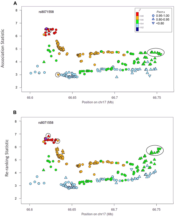
Re-ranking identifies new top SNPs for 2 of the 3 associated loci: 8q24.21 and 17q24.3 (Figures 4 and 5 respectively). In addition to the most significant region at 8q24.21 (Figure 4), re-ranking also identifies a new top SNP for the third most significant region (Figure S11). For both regions re-ranking also identifies SNPs that may have otherwise been missed due to imperfect imputation. After re-ranking, 2 SNPs in the most significant region at the 8q24.21 locus (Figure 4) and 8 SNPs at the 17q24.3 locus (Figure 5) move from the lower ranks into the top 10 percent. On the other hand, SNPs in the top 10% are moved down by only a few ranks. In this way, re-ranking keeps highly significant SNPs identified by the naïve ranking and adds a few SNPs that would have otherwise been missed. When the top test statistics are of similar size, re-ranking may identify a new top SNP. When most SNPs are well-genotyped, re-ranking makes only subtle changes (Figure S11, S12 and S13).
There is one poorly imputed SNP at 17q24.3 (rs1014000, r2 = 0.20) that moves from the naïve rank of 245 to the new rank of 16 after adjustment. This SNP's apparent association is largely driven by data from a single study: the naïve rank in the EPIC study is 10. When we remove this study from the meta-analysis, the naïve rank is 306 and the adjusted rank is 119. No other SNP in the top 10% is this drastically affected when the EPIC study is removed from the analysis. In the meta-analysis context, we recommend examining top SNPs for heterogeneity among studies when re-ranking produces dramatically different results.
Discussion
Overall, we observed that the tagging and genotyping accuracy effects are non-trivial sources of bias that could obscure association evidence at the causal SNP. The proposed re-ranking procedure is simple to implement and can substantially increase the probability of identifying the causal SNP. For low-coverage sequencing, we recommend the re-ranking method to improve causal SNP identification. For imputation and high-coverage sequencing, we recommend that unfiltered SNPs in associated regions be examined to see if correlation varies across SNPs and if so, we recommend adjustment with the re-ranking method. Large changes in rank should be carefully examined for underlying issues such as heterogeneity among meta-analysis studies or differential accuracy between cases and controls, and procedures to correct for these issues should be incorporated.
Re-ranking is most beneficial when genotyping accuracy is moderate to low, that is, the average correlation between the actual and estimated genotypes of post-GWAS (sequenced or imputed) SNPs is less than 0.97. A large number of post-GWAS SNPs in a study may appear to be significant, but when not all were directly genotyped with high accuracy, re-ranking can help select the most probable causal SNPs for follow-up. High density genotyping followed by low-coverage sequencing in the same sample can produce misleading results, as demonstrated by our simulations, so we do not recommend this design for identifying causal variants. Our re-ranking method tends to down-rank the tag SNP. If the tag SNP is suspected to be causal (e.g. based on prior study), we recommend examining the rank of the tag SNP using both the naïve and re-ranked methods when selecting SNPs for further study. Several imputation and sequencing software packages provide accurate estimates of ρ or quantities from which ρ can be computed [24], [39]. Re-ranking depends on accurate estimates of ρ. Recalibration of sequencing quality scores can greatly improve accuracy and so we recommend this step prior to re-ranking [27].
Re-ranking is especially important when study-specific factors exacerbate the effects of GWAS-based selection and genotyping error. Such factors include: high genetic diversity which makes sequencing reads difficult to align [27]; low LD among SNPs or lack of population-specific reference panels which makes some populations particularly difficult to impute (e.g. some African populations [50]); and imputation error which can be as high as 10% for these populations. Low MAF SNPs tend to suffer from both low power (which exacerbates the tagging effect) and high genotyping error. Re-ranking can be applied to rare and low MAF SNPs with allele counts large enough for test statistics to reach asymptotic normality. Very low (1×−2×) and extremely low (0.1×−0.5×) read depth sequencing has received recent attention as a way to maximize cost efficiency and make use of off-target sequencing data [29], [32]. Error rates for such regions would be both very high and highly variable among SNPs and so re-ranking to account for errors in the estimated genotypes would be crucial. When genotyping accuracy is extremely poor, the re-ranking method may not be able to sufficiently improve the localization success rate to ensure useful results. We recommend that investigators consider the accuracy thresholds recommended by the genotype calling or imputation algorithm they are using before re-ranking is applied.
We emphasize that re-ranking improves the localization success rate when applied to SNPs under the alternative, i.e. SNPs that are themselves causal or in LD with a causal SNP. Including null SNPs in the re-ranking procedure increases the number of SNPs the causal must out-compete, and so we recommend that only SNPs suspected to be under the alternative be included. In our application we included all SNPs that had squared pairwise correlation (r2) with the index SNP (most significant SNP in the region) greater than 0.2.
Existing methods that incorporate genotype uncertainty into tests for association to reduce power lost due to genotyping error or missing data [e.g. 51]–[54] do not completely recover lost power, and so the genotyping accuracy effect will remain. The simplest way to deal with genotype uncertainty in a test is to use the expected additive genotype (i.e. the posterior mean or dosage) in the standard linear or logistic regression. In this case, the re-ranking method can be applied using the allele dosages in place of called genotypes as described above. Guan and Stephens [55] compared several frequentist and Bayesian methods that incorporate genotype uncertainty into tests for association. The re-ranking procedure could be extended to any case where the correlation between test statistics or Bayes factors can be worked out.
We expect that re-ranking will play an important role as sequencing costs fall and GWAS platform coverage increases. Ultra-high density GWAS platforms are more likely to include tag SNPs in very high correlation with the causal SNP, which increases power to detect indirect association at the tag SNP. However, without re-ranking, strong tagging also decreases power to correctly identify the causal SNP in subsequent low-coverage sequencing. Advances in GWAS and sequencing platforms will allow researchers to drill down into lower MAFs and smaller effect sizes. Both low MAF and small effect size yield lower power, which exacerbates upward bias at the tag [20] and, therefore, the adverse tagging effect. Low MAF SNPs tend to suffer from higher error rates, which exacerbates the genotyping accuracy effect. Association study sample sizes will therefore need to continue to increase, so even as sequencing costs fall, it is anticipated that low-coverage will continue to be the most cost-effective design for many studies, despite the high genotyping error rates [27]. In conclusion, we anticipate that re-ranking to correct for the adverse effects of selection, tagging and differential genotyping accuracy rates among SNPs will continue to be important in candidate causal SNP identification for some time.
Supporting Information
Zdroje
1. CooperGM, ShendureJ (2011) Needles in stacks of needles: finding disease-causal variants in a wealth of genomic data. Nat Rev Genet 12 : 628–40.
2. GeorgesM (2011) The long and winding road from correlation to causation. Nat Genet 43(3): 180–1.
3. IoannidisJP, ThomasG, DalyMJ (2009) Validating, augmenting and refining genome-wide association signals. Nat Rev Genet 10 : 318–29.
4. ZaitlenN, PaşaniucB, GurT, ZivE, HalperinE (2010) Leveraging genetic variability across populations for the identification of causal variants. Am J Hum Genet 86 : 23–33.
5. UdlerMS, TyrerJ, EastonDF (2010) Evaluating the power to discriminate between highly correlated SNPs in genetic association studies. Genet Epidemiol 34(5): 463–8.
6. HolmH, GudbjartssonDF, SulemP, MassonG, HelgadottirHT, et al. (2011) A rare variant in MYH6 is associated with high risk of sick sinus syndrome. Nat Genet 43(4): 316–320.
7. ZegginiE (2011) Next-generation association studies for complex traits stopping RNA interference at the seed. Nat Genet 43 : 287–288.
8. Kang HM, Gaulton K,Voight BF, Fuchsberger C, Pearson RD, et al.. (2011) Sequencing and genotyping thousands of European genomes and exomes to better understand the genetic architecture of type 2 diabetes: the GoT2D study [Abstract 190]. In: 61st Annual American Society of Human Genetics Program Book; 11–15 October 2011; Montreal, Quebec, Canada. Available: www.ichg2011.org/program_guide.
9. HuZ, XiaY, GuoX, DaiJ, LiH, et al. (2011) A genome-wide association study in Chinese men identifies three risk loci for non-obstructive azoospermia. Nat Genet 44(2): 183–186.
10. TenesaA, FarringtonSM, PrendergastJG, PorteousME, WalkerM, et al. (2008) Genome-wide association scan identifies a colorectal cancer susceptibility locus on 11q23 and replicates risk loci at 8q24 and 18q21. Nat Genet 40(5): 631–7.
11. FridleyBL, AboR, BrisbinA, JenkinsGD (2011) Sample selection study designs to follow-up GWAS signals with targeted sequencing. Genet Epidemiol 36 : 148.
12. O'DonovanMC, CraddockN, NortonN, WilliamsH, PeirceT, et al. (2008) Identification of loci associated with schizophrenia by genome-wide association and follow-up. Nat Genet 40(9): 1053–5.
13. Wellcome Trust Case Control Consortium (2007) Genome-wide association study of 14,000 cases of seven common diseases and 3,000 shared controls. Nature 447(7145): 661–78.
14. WiltshireS, MorrisAP, ZegginiE (2008) Examining the statistical properties of fine-scale mapping in large-scale association studies. Genet Epidemiol 32 : 204–14.
15. Beavis WD. (1994) The power and deceit of QTL experiments: lessons from comparative QTL studies. In: Proceedings of the Forty-Ninth Annual Corn & Sorghum Industry Research Conference. American Seed Trade Association: Washington, DC, United States.
16. GöringHH, TerwilligerJD, BlangeroJ (2001) Large upward bias in estimation of locus-specific effects from genomewide scans. Am J Hum Genet 69 : 1357–1369.
17. SunL, BullSB (2005) Reduction of selection bias in genome-wide genetic studies by resampling. Genet Epidemiol 28 : 352–367.
18. GarnerC (2007) Upward bias in odds ratio estimates from genome-wide association studies. Genet Epidemiol 31 : 288–295.
19. BowdenJ, DudbridgeF (2009) Unbiased estimation of odds ratios: combining genomewide association scans with replication studies. Genet Epidemiol 33(5): 406–18.
20. FayeLL, BullSB (2011) Two-stage study designs combining genomewide association studies, tag single-nucleotide polymorphisms, and exome sequencing: accuracy of genetic effect estimates. BMC Proceedings 5(Suppl 9): S64.
21. OssowskiS, SchneebergerK, ClarkRM, LanzC, WarthmannN, et al. (2008) Sequencing of natural strains of Arabidopsis thaliana with short reads. Genome Res 18 : 2024–2033.
22. HarismendyO, NgPC, StrausbergRL, WangX, StockwellTB, et al. (2009) Evaluation of next generation sequencing platforms for population targeted sequencing studies. Genome Biol 10: R32.
23. PoolJE, HellmannI, JensenJD, NielsenR (2010) Population genetic inference from genomic sequence variation. Genome Res 20 : 291–300.
24. LiY, Willer CJ, DingJ, ScheetP, AbecasisGR (2010) MaCH: using sequence and genotype data to estimate haplotypes and unobserved genotypes. Genet Epidemiol 34(8): 816–34.
25. LiY, SidoreC, KangHM, BoehnkeM, AbecasisG (2011) Low-coverage sequencing: Implications for the design of complex trait association studies. Genome Res 21 : 940–951.
26. LuoL, BoerwinkleE, XiongM (2011) Association studies for next-generation sequencing. Genome Research 21 : 1099–108.
27. NielsenR, PaulJS, AlbrechtsenA, SongYS (2011) Genotype and SNP calling from next-generation sequencing data. Nat Rev Genet 12(6): 443–51.
28. MechanicLE, ChenHS, AmosCI, ChatterjeeN, CoxNJ, et al. (2011) Next generation analytic tools for large scale genetic epidemiology studies of complex diseases. Genet Epidemiol 35 : 22–35.
29. PasaniucB, RohlandN, McLarenPJ, GarimellaK, ZaitlenN, et al. (2012) Extremely low-coverage sequencing enables cost effective GWAS. Nat Genet 44 : 631–635.
30. JohnsonPLF, SlatkinM (2008) Accounting for bias from sequencing error in population genetic estimates. Mol Bio Evol 25 : 199–206.
31. 1000 Genomes Project (2010) A map of human genome variation from population-scale sequencing. Nature 467(7319): 1061–73.
32. SampsonJ, JacobsK, YeagerM, ChanockS, ChatterjeeN (2011) Efficient study design for next generation sequencing. Genet Epidemiol 277 : 269–277.
33. KimSY, LiY, GuoY, LiR, HolmkvistJ, et al. (2010) Design of association studies with pooled or un-pooled next-generation sequencing data. Genet Epidemiol 34 : 479–91.
34. BlowN (2009) Genomics: Catch me if you can. Nat Methods 6(7): 539–544.
35. ZaitlenN, EskinE (2010) Imputation aware meta-analysis of genome-wide association studies. Genet Epidemiol 34 : 537–542.
36. GarnerC (2011) Confounded by sequencing depth in association studies of rare alleles. Genet Epidemiol 35 : 261–268.
37. SinnottJA, KraftP (2012) Artifact due to differential error when cases and controls are imputed from different platforms. Hum Genet 131 : 111–9.
38. MachielaMJ, ChenC, LiangL, DiverRW, StevensVL, et al. (2013) One thousand genomes imputation in the National Cancer Institute Breast and Prostate Cancer Cohort Consortium aggressive prostate cancer genome-wide association study. Prostate 73(7): 677–89.
39. BrowningBL, BrowningSR (2009) A unified approach to genotype imputation and haplotype-phase inference for large data sets of trios and unrelated individuals. Am J Hum Genet 84(2): 210–23.
40. FayeLL, SunL, DimitromanolakisA, BullSB (2011) A flexible genome-wide bootstrap method that accounts for ranking and threshold-selection bias in GWAS interpretation and replication study design. Stat Med 30 : 1898–1912.
41. SunL, DimitromanolakisA, FayeLL, PatersonAD, WaggottD, et al. (2011) BR-squared: a practical solution to the winner's curse in genome-wide scans. Hum Genet 129(5): 545–52.
42. ZhongH, PrenticeR (2008) Bias-reduced estimators and confidence intervals for odds ratios in genome-wide associationstudies. Biostatistics 9 : 621–634.
43. GhoshA, ZouF, WrightF (2008) Estimating odds ratios in genome scans: an approximate conditional likelihood approach. Am J Hum Genet 82 : 1064–1074.
44. XiaoR, BoehnkeM (2009) Quantifying and correcting for the Winner's curse in genetic association studies. Genet Epidemiol 33 : 453–462.
45. ZollnerS, PritchardJK (2007) Overcoming the winner's curse: estimating penetrance parameters from case-control data. Am J Hum Genet 80 : 605–615.
46. XuL, CraiuRV, SunL (2011) Bayesian methods to overcome the winner's curse in genetic studies. Ann Appl Stat 5(1): 201–31.
47. BrowningBL, YuZ (2009) Simultaneous genotype calling and haplotype phasing improves genotype accuracy and reduces false-positive associations for genome-wide association studies. Am J Hum Genet 85(6): 847–61.
48. SchumacherFR, BerndtSI, SiddiqA, JacobsKB, WangZ, et al. (2011) Genome-wide association study identifies new prostate cancer susceptibility loci. Hum Mol Genet 20 : 3867–75.
49. ChungCC, CiampaJ, YeagerM, JacobsKB, BerndtSI, HayesRB, et al. (2011) Fine mapping of a region of chromosome 11q13 reveals multiple independent loci associated with risk of prostate cancer. Human Molecular Genetics 20(14): 2869–78.
50. HuangL, WangC, RosenbergNA (2009) The relationship between imputation error and statistical power in genetic association studies in diverse populations. Am J Hum Genet 85(5): 692–8.
51. HaoK, WangX (2004) Incorporating individual error rate into association test of unmatched case-control design. Hum Hered 58 : 154–63.
52. LinDY, HuY, HuangBE (2008) Simple and efficient analysis of disease association with missing genotype data. Am J Hum Genet 82 : 444–452.
53. MarchiniJ, HowieB, MyersS, McVeanG, DonnellyP (2007) A new multipoint method for genome-wide association studies by imputation of genotypes. Nat Genet 39(7): 906–13.
54. AcarEF, SunL (2013) A generalized Kruskal-Wallis test incorporating group uncertainty with application to genetic association studies. Biometrics in press.
55. GuanY, StephensM (2008) Practical issues in imputation-based association mapping. PLoS Genet 4(12): e1000279.
Štítky
Genetika Reprodukční medicínaČlánek vyšel v časopise
PLOS Genetics
2013 Číslo 8
- Kazuistika – Perspektivy využití precizované medicíny v rámci personalizované specifické terapie onkologických pacientů
- Nobelova cena za chemii pro genetické nůžky: Objev, který změní naši budoucnost?
- Technologie na bázi RNA v klinické praxi: od přebarvených petúnií k terapii vzácných a dosud jen obtížně léčitelných chorob u lidí
- „Nepředstavovali jsme si, že náš výzkum povede přímo ke vzniku nových léků, dokonce ještě za našeho života“
- Bezplatné služby pro diagnostiku ATTRv amyloidózy pro kardiology
Nejčtenější v tomto čísle
- Chromosomal Copy Number Variation, Selection and Uneven Rates of Recombination Reveal Cryptic Genome Diversity Linked to Pathogenicity
- Genome-Wide DNA Methylation Analysis of Systemic Lupus Erythematosus Reveals Persistent Hypomethylation of Interferon Genes and Compositional Changes to CD4+ T-cell Populations
- Associations of Mitochondrial Haplogroups B4 and E with Biliary Atresia and Differential Susceptibility to Hydrophobic Bile Acid
- A Role for CF1A 3′ End Processing Complex in Promoter-Associated Transcription
Zvyšte si kvalifikaci online z pohodlí domova
Mazová zátka a její řešení
nový kurzVšechny kurzy