
A Multi-Trait, Meta-analysis for Detecting Pleiotropic Polymorphisms for Stature, Fatness and Reproduction in Beef Cattle
We describe novel methods for finding significant associations between a genome wide panel of SNPs and multiple complex traits, and further for distinguishing between genes with effects on multiple traits and multiple linked genes affecting different traits. The method uses a meta-analysis based on estimates of SNP effects from independent single trait genome wide association studies (GWAS). The method could therefore be widely used to combine already published GWAS results. The method was applied to 32 traits that describe growth, body composition, feed intake and reproduction in 10,191 beef cattle genotyped for approximately 700,000 SNP. The genes found to be associated with these traits can be arranged into 4 groups that differ in their pattern of effects and hence presumably in their physiological mechanism of action. For instance, one group of genes affects weight and fatness in the opposite direction and can be described as a group of genes affecting mature size, while another group affects weight and fatness in the same direction.
Published in the journal:
. PLoS Genet 10(3): e32767. doi:10.1371/journal.pgen.1004198
Category:
Research Article
doi:
https://doi.org/10.1371/journal.pgen.1004198
Summary
We describe novel methods for finding significant associations between a genome wide panel of SNPs and multiple complex traits, and further for distinguishing between genes with effects on multiple traits and multiple linked genes affecting different traits. The method uses a meta-analysis based on estimates of SNP effects from independent single trait genome wide association studies (GWAS). The method could therefore be widely used to combine already published GWAS results. The method was applied to 32 traits that describe growth, body composition, feed intake and reproduction in 10,191 beef cattle genotyped for approximately 700,000 SNP. The genes found to be associated with these traits can be arranged into 4 groups that differ in their pattern of effects and hence presumably in their physiological mechanism of action. For instance, one group of genes affects weight and fatness in the opposite direction and can be described as a group of genes affecting mature size, while another group affects weight and fatness in the same direction.
Introduction
Polymorphisms that affect complex traits (quantitative trait loci or QTL) may affect multiple traits. This pleiotropy is the main cause of the genetic correlations between traits, although another possible cause of genetic correlation is linkage disequilibrium (LD) between the QTL for different traits. A positive genetic correlation that is less than 1.0 between two traits, such as weight and fatness, implies that some QTL affect both traits in the same direction, but other QTL may affect only one trait and a small number may even affect the traits in the opposite direction. Identifying QTL with different patterns of pleiotropy should help us to understand the physiological control of multiple traits. Although genome wide association studies (GWAS) are usually performed one trait at a time, it is not uncommon to find that two traits are associated with SNPs in the same region of a chromosome. This has been described as cross phenotype association [1]. Resolving whether cross phenotype associations are due to one QTL with pleiotropic effects or two linked QTL [1] has proved challenging, given the large number of loci that appear to cause variation in complex traits [2]–[5].
In practice, the apparent effect of a SNP on a trait is estimated with some experimental or sampling error. Consequently, even if there is a single QTL in a region of the chromosome, the SNP with the strongest association may vary from one trait to another causing the estimated position of the QTL to vary between traits. If one QTL can explain the findings for the multiple traits then a multi-trait analysis might result in higher power to detect QTL and greater precision in mapping them. Multiple-trait analysis of linkage experiments has been reported to increase the power to detect QTL [6], [7]. This paper investigates whether additional power can be extracted from a GWAS by analyzing traits together rather than one at a time.
In principle, provided the computing power exists, a multi-trait GWAS is statistically straightforward. However, typically not all subjects have been measured for all traits, and when different traits have been investigated in different experiments, the individual subject data may not even be available. Therefore we present an approximate, multi-trait meta-analysis that uses as data the estimated effects of the SNPs from n individual trait GWAS.These effects are expressed as a vector of signed t-values (t) and the error covariance matrix of these t values is approximated by a n×n correlation matrix of t-values among the traits calculated across the SNP (V). Consequently, t'V−1t is approximately distributed as a chi-squared with n degrees of freedom. The meta-analysis used here, although approximate, appropriately models the variances and covariance among the t-values regardless of the overlap in individuals measured for the different traits. The different amount of information for the different traits (e.g. different number of individuals genotyped, size of error variance relative to SNP effect) is accounted for in the analysis.
To distinguish between pleiotropy and multiple, linked QTL, we use two different analyses. Firstly, we consider whether all SNPs in a region do or do not show the same pattern of effects across traits. Secondly, we fit the most significant SNP from the multi-trait analysis in the model to test whether this does or does not eliminate the evidence for a second QTL.
An aim of GWAS is to identify the genes and polymorphic sites in the genome that cause variation in complex traits. Choosing the most likely candidate genes from the region surrounding a SNP is usually based on the relationship between the function of the gene and the trait. Assuming that some QTL show pleiotropy, the pattern of pleiotropic effects would be an important clue to the nature of the causative mutation and the function of the gene in which it occurred. Genes that belong to the same pathway might have a similar pattern of pleiotropic effects. Therefore we investigate whether QTL can be clustered into groups with a similar pattern of pleiotropic effects and hence into physiologically similar groups.
The objectives of this study were to test the power of a multi-trait, meta-analysis to detect and map pleiotropic QTL affecting growth, feed conversion efficiency, carcass composition, meat quality and reproduction in beef cattle. We also investigate whether these pleiotropic QTLs can be placed in groups with a similar pattern of effects and hence similar underlying physiological mechanisms.
Results
Power of multi-trait meta-analysis to detect QTL
False discovery rate
In this study, the 10,191 cattle had real or imputed genotypes for 729,068 SNP, although not all cattle were measured for all traits. The cattle were sourced from 9 different populations (Angus, Murray Grey, Shorthorn, Hereford, Brahman, Belmont Red, Santa Gertrudis, Tropical composites, and recent Brahman crosses). Single trait genome wide association studies were performed for the 32 traits listed in Table 1 and the results have been previously reported by Bolormaa et al. [8]. The traits include measures at different ages of height, weight, fatness, muscularity, feed intake, meat tenderness, age at puberty, and interval of postpartum anoestrus (Table 1).

In the multi-trait analysis we measured the effect of a SNP on each trait by a signed t-value (effect/standard error of effect) and approximated the (co)variance matrix among the traits using the correlation matrix of these SNP effects. Then the effects of a SNP across the 32 traits were combined with this correlation matrix to perform a multi-trait chi-squared test with 32 degrees of freedom of the null hypothesis that a SNP has no effect on any trait.
For this test, 2,028 SNPs were significant (P<5×10⁻⁷) (Figure 1). This corresponds to a false discovery rate (FDR) of 0.02%, and this was lower than for any individual trait; when traits were analyzed individually, for 19 out of 32 traits the FDR at P<5×10⁻⁷ ranged from 0.04% to 2.5% and for the 13 remaining traits FDR was greater than 3.5% (Table 2). Therefore the multi-trait test had greater power to detect QTL than the individual trait analyses.


Validation of SNP effects
To validate the associations found in the multi-trait analysis, we used individual level data. The data were split into a discovery sample and a validation sample. The whole data were split into five sets by allocating all of the offspring of randomly selected sires to one of the five datasets. Then one of the 5 divisions was randomly selected as a validation population and the other 4 divisions as the reference population. In this way no animal used for validation had paternal half sibs in the reference population.
From the multi-trait analysis of the discovery dataset, the most significant SNPs (P<10−5) were retained and then to avoid identifying a large number of closely linked SNPs whose association with traits is due to the same QTL, only the most significant SNP in a 1 Mb interval was selected for validation.
For each SNP we calculated the linear index of 22 traits. This linear index had maximum correlation with the corresponding SNP. Then the association between a SNP and its corresponding linear index was tested in the validation sample. To do this we needed individual animals that had been measured for nearly all traits. However, the bulls and cows, which had been measured for 10 reproductive traits, were not measured for the other 22 traits. Therefore we based the validation on animals measured for the 22 non-reproductive traits and calculated the linear index for each SNP based on these 22 traits (Table 3). Out of the 244 significant SNPs, 207 or 85% had an effect in the same direction in the validation sample as in the discovery sample. The size of the validation sample (1,899 animals) limited its power but 72 of the 244 SNPs were significant (P<0.05) and 71 of the 72 had an effect in the same direction as in the discovery sample.
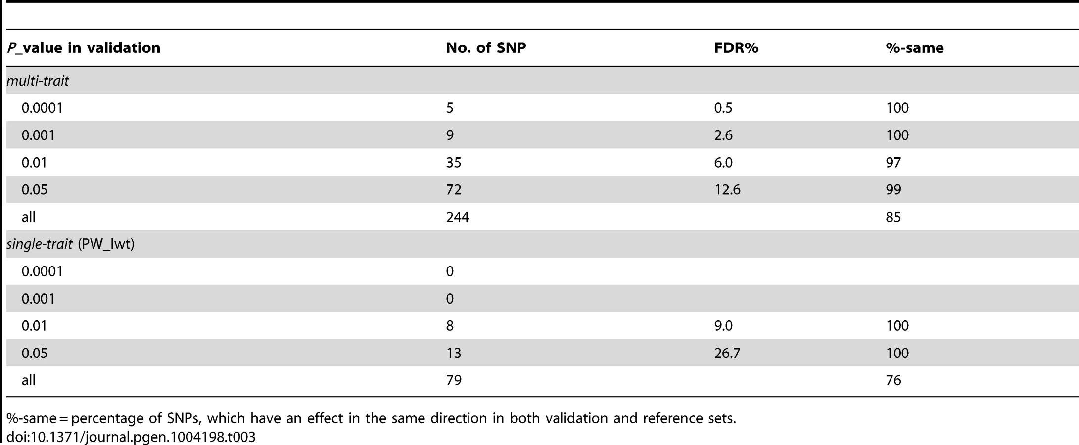
To compare the power of detecting QTL in the multi-trait analysis to that in the single-trait analysis, we performed the same validation analysis for the single trait post weaning live weight (PW_lwt), which is one of the traits with the highest number of significant associations (Table 3). For PW_lwt, only 79 SNP met the criterion (P<10−5 and one SNP per Mb) and of these 60 (76%) had an effect in the same direction in the validation sample as in the discovery sample, but only 13 of the 79 were significant at P<0.05 in the validation sample. This shows that multi-trait analysis detected more associations and validated a higher percentage of them than the best single trait analysis. For other single traits the proportion of significant SNPs from the reference that were validated was even lower than for PW_lwt.
Precision of multi-trait meta-analysis for QTL mapping
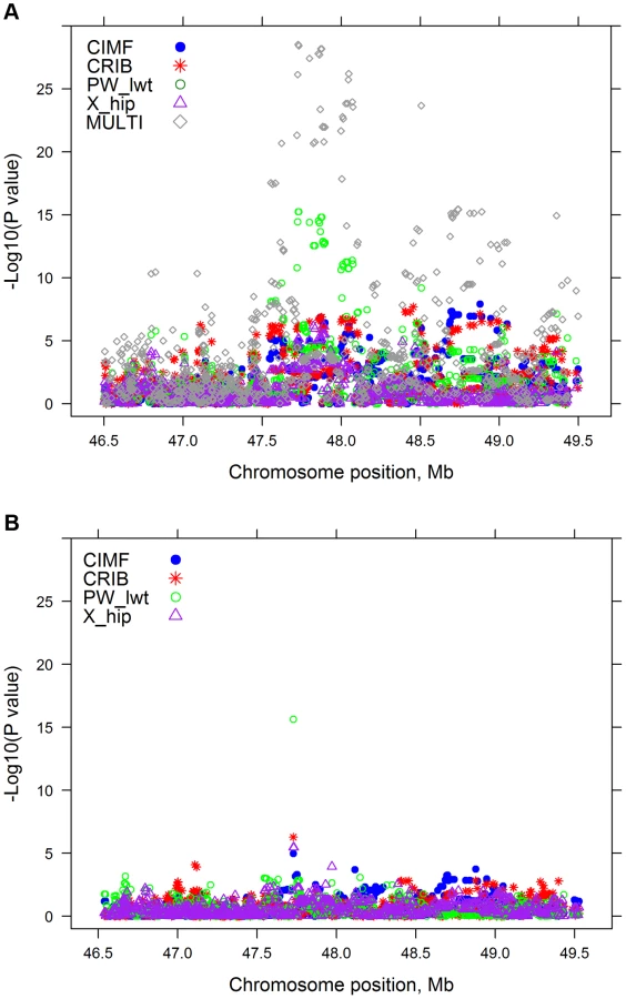
Many of the significant SNPs in both single trait and multi-trait analyses were linked and might be associated with the same QTL. As an example of the multi-trait approach to improve precision, Figure 2A shows the significance of SNP effects for 4 single trait GWAS and our multi-trait statistic in a region of chromosome 5 (BTA 5). The 4 separate traits map the QTL to slightly different positions (range: 47,732–48,877 kb). For the multi-trait statistic, based on SNP effects from single-trait GWAS for 32 traits, the most significant SNP (P = 1.32×10⁻²⁷) was located at 47,728 kb. The multi-trait analysis represents a good compromise between the positions from the 4 single trait GWAS and may be the best guide to a single QTL position explaining all the associated traits.
Multi-trait meta-analysis tends to find SNPs near genes
SNPs were classified according to their distance from the nearest gene and the proportion of SNPs at each distance from a gene that were significant (P<10−5) in the multi-trait analysis was calculated. Figure 3 shows that SNPs were more likely to be significantly associated with the 32 traits if they were within or less than 100 kb from a gene.

Single-trait GWAS to test pleiotropy or linkage
There are many regions of the genome, similar to that illustrated in Figure 2A, where multiple traits had significant associations with one or more SNPs. For each SNP their estimated effects on each trait were expressed as a signed t-value. For each pair of SNPs we calculated the correlation across the 32 traits between their estimated effects so that SNPs with the same pattern of effects across traits are highly positively or negatively correlated. Figure 4 shows the correlation between SNPs on a region of chromosomes 7 and 14. All SNPs in the vicinity of 25 Mb on chromosome 14 are highly correlated indicating a single pleiotropic QTL in this region, corresponding to previous reports of a polymorphism near the gene PLAG1 that affects many traits [9]–[11]. On chromosome 7 there are three blocks of SNPs with high correlations within a block and low correlations between blocks suggesting there are three QTL, close to 93, 95 and 98 Mb. The QTL at 98 Mb corresponds to a previously reported polymorphism in calpastatin (CAST) [12], [13]. Below, we confirm this interpretation by fitting the most significant SNPs in the model and testing for additional associations.

Conditional analyses to test pleiotropy or linkage
Detection of pleiotropic QTL
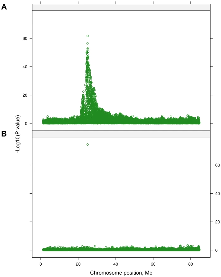
Many highly significant SNPs from the multi-trait analyses were found within narrow regions on chromosomes (BTA) 3, 5, 6, 7, 14, 20 and 29 (Figure 1). If there is only a single QTL in a region and if it is perfectly tagged by one of the SNPs, then when this SNP is fitted in the model the other nearby SNPs should have no significant association with the phenotypes. To test this hypothesis we selected 28 ‘lead’ SNPs (Table 4), representing what appeared to be 28 QTL across the genome. GWAS were re-performed but the SNPi (SNPi, i = 1, 2, 3, …, 729068) along with the 28 lead SNPs were simultaneously fitted in the model, and then the multi-trait statistic was re-calculated for SNPi to test the effects of the SNPi across traits after fitting the 28 lead SNPs. Figure 5 shows the results for BTA 14 as an example. In the original multi-trait GWAS, many SNPs between 20 and 40 Mb on BTA 14 were significant but after fitting the 28 lead SNPs, which include one at 25 Mb on BTA 14, there were no more significant SNPs in this region than in the rest of BTA 14 (Figure 5 shows the lead SNP as well as all other SNPs).

All 28 lead SNPs remained significant in this conditional analysis, even after fitting the other 27, showing that each tags a different QTL. For instance, on BTA 7 the 2 lead SNPs at 93 and 98 Mb remain significant as does a SNP at 95 Mb (Figure 6). This confirms the interpretation of the correlation analysis (Figure 4) that there are 3 QTL in this narrow region. The apparent effects of the 28 lead SNPs on the 32 traits, as estimated in the original single-trait GWAS, are given in Table 5 (only values with |t|>1 are reported).


In some cases, a SNP close to the lead SNP remains significant even after fitting the 28 lead SNPs. This could be because of imperfect LD between the lead SNP and the causal mutation so that other SNP may explain some of the variance caused by the causal mutation in addition to the lead SNP. Alternatively, there may be more than one causal variant in the same gene each tracked by a different SNP. In fact, there were still many significant SNPs (P<5×10⁻⁷) scattered throughout the genome (eg., there were 62 significant SNPs for PW_hip; Table 2) indicating that there are likely to be many more than 28 QTL affecting these 32 traits.
Mapping of pleiotropic QTL
In Figure 2B the significance of SNP effects for 4 single trait GWAS in a region of chromosome 5 is presented, when the ith SNP (SNPi, i = 1,2,3, …, 729068) along with 28 lead SNPs were simultaneously fitted in the GWAS model. The results from this conditional analysis show that the lead SNP is significant (P<10−5) for all 4 traits, but once this SNP is included in the model, no other nearby SNPs reach this level of significance for any of the 4 traits.
Clustering of QTL with similar pattern of effects across traits
For each pair of SNPs among the 28 lead SNPs, the correlation of their effects across the 32 traits was calculated (Figure 7). There are a few correlations with high absolute value, such as between the lead SNPs on BTA 5, 6 and 14, but most correlations are low. A low correlation suggests QTL with different patterns of effects across traits, however sampling errors in estimating SNP effects also reduce the absolute value of the correlation. If two QTL affect the same physiological pathway one might expect them to have the same pattern of effects and hence a high correlation. Cluster analysis based on effects of the SNPs across traits divided the 28 lead SNPs into 4 loosely defined groups (Figure 7), which share patterns of effects across traits (although there are still differences within each group in the exact pattern of effects across traits) (Table 5).

Group 1 consists of 4 lead SNPs located on BTA 5 (BTA5_47.7 Mb), 6 (BTA6_40.1 Mb), 14 (BTA14_25.0 Mb) and 20 (BTA20_4.9 Mb). This group clustered as an outer branch separate from the other 24 lead SNPs (Figure 7), indicating that this group of SNPs clusters more tightly than the other groups. Three of these 4 SNPs were highly correlated amongst each other while the SNP on BTA 20 had slightly lower correlations to the other 3 SNPs. Table 5 shows that these 4 SNPs have an allele that increases height and weight and decreases fatness, RFI and blood concentration of IGF1. They could be described as changing mature size.
Group 2 consists of SNPs on BTA 7 (BTA7_98 Mb), 10 (BTA10_92 Mb), 25 (BTA25_3.7 Mb), 26 (BTA26_28.0 Mb), and 29 (BTA29_44.8 Mb) with high correlations between 2 SNP on BTA 7 and 29. These SNPs have an allele that increases meat tenderness (i.e., decrease shear force) and fatness (i.e., marbling or intra-muscular fat) (Table 5). The SNPs at BTA7_98.5 Mb and BTA29_45.8 Mb have a large effect on shear force and map to the positions of known genes affecting this trait (Calpastatin and Calpain 1) [12], [14], [15].
Group 3 consists of 7 SNPs that are located on BTA 2 (BTA2_25.2 Mb), 3 (BTA3_80.1 Mb), 6 (BTA6_12.7 Mb), 13 (BTA13_34.9 Mb), 17 (BTA17_24.9 Mb), 19 (BTA19_25.1 Mb), and 25 (BTA25_14.5 Mb). There was weaker clustering and lower correlations between these SNP compared to groups 1 and 2. The SNPs of Group 3 have an allele that increases both fatness and weight but has little effect on height or IGF1 (Table 5). This distinguishes these SNPs from those in Group 1 where the allele that increases weight also decreases fatness and IGF1.
Group 4, the biggest group, consists of 12 SNPs in a loose cluster. Moderate correlations appeared between some SNPs on BTA 7 (BTA7_93.2 Mb), 9 (BTA9_100.5 Mb), 21 (BTA21_0.9 Mb), 21 (BTA21_19.0 Mb), 23 (BTA23_43.9 Mb), 4 (BTA4_77.6 Mb) and 8 (BTA8_59.2 Mb) (Figure 7). This group has an allele that tends to increase muscling, retail beef yield (RBY), tenderness and feed efficiency, and decrease fatness. The clustering did separate the 2 SNPs on BTA 7 with the SNP near 98 Mb belonging to Group 2 and the SNP near 93 Mb belonging to Group 4.
Although the SNPs within a group share some features they also differ in some of their associations. For instance, in Group 1 the SNP on BTA 14 near PLAG1 has a more marked effect on age at puberty (AGECL) than others in the group; the SNP on BTA5 changes the distribution of fat between the P8 site on the rump and rib site and the intramuscular depot. Thus it is possible for the each SNP to have a unique pattern of associations with phenotypic traits.
Finding additional QTL in the same pathway
The pattern of pleiotropic effects might be an important clue to the nature of the causative mutation and the function of the gene in which it occurred. Genes that operate in the same pathway might be expected to show the same pattern of pleiotropic effects. For each of the 28 lead SNPs, we searched for additional SNPs with a similar pattern of effects. To do this we used the linear index of 22 traits that showed the highest association with a lead SNP, as previously defined for validation of the multi-trait analysis, and performed a new GWAS using the linear index as a new trait. Table 6 shows the number of significant (P<10−5) SNPs for the 28 linear indexes corresponding to the 28 lead SNPs. Out of 28 linear indexes, 19 had more than 70 significant SNPs and hence a FDR of less than 10%. Linear index BTA5_47.7 Mb, BTA6_40.1 Mb, BTA14_25.0 Mb, and BTA20_4.9 Mb (where the name corresponds to the location of the QTL defining the pattern of effects) have associations with over 1,000 significant SNPs across the genome. For the index based on the lead SNP BTA5_47.7 Mb, the significant SNPs included 615 SNPs on BTA 5, 64 on BTA 6, 24 on BTA 11, 907 on BTA 14, 19 on BTA 17, 18 on BTA 20. This reiterates the result obtained in the cluster analysis because SNPs on BTA 5, 6, 14 and 20 are the lead SNPs in Group 1 and the additional SNPs on these chromosomes may be tagging the same QTL as the lead SNPs. However, there are also significant SNPs associated with this linear index on BTA 11, 17, 19, 21 and 25.

The additional significant SNPs were assigned to the 4 groups as follows. For each SNP, the linear index with which it showed the most significant association (P<5×10⁻⁷) was found. The SNP was then assigned to the same group as the lead SNP defining that linear index. The results are shown in Figure 8. Usually this procedure identified a set of closely linked SNPs, presumably indicating a single QTL. Therefore we kept in the final group only the most significant SNP (P<5×10⁻⁷) from each set. The number of significant SNPs assigned to each of the 4 Groups were as follows: 1) 2,076; 2) 398; 3) 169 and 4) 176. The positions or regions of the most significant SNPs in the expanded groups are listed in Table 7.


Candidate genes
For each SNP or group of SNPs in Table 7 we examined the genes within 1 Mb and, in some cases, identified a plausible candidate for the phenotypic effect (Table 7). Focusing on those regions with multiple SNPs, the genes CAPN1, CAST, and PLAG1, were again identified, which are strongly identified with meat quality and growth in previous cattle studies [16]–[18]. In addition, we identified the genomic regions that include the HMGA2, LEPR, DAGLA, ZEB1, IGFBP3, FGF6 and ARRDC3 genes as having strong genetic effects in cattle. HMGA2 and LEPR are well known to have effects on fatness and body composition in pigs [19], [20]. SNP in the promoter of IGFBP3 have been shown to affect the level of IGFBP3 in humans, which affects availability of circulating IGF1 and has a multitude of effects on growth and development [21]. Here we show a strong effect for IGFBP3, where previous results for marbling or backfat have either been small or non-significant [22], [23]. Differences in gene expression of FGF6 has been shown to be associated to muscle development in cattle [24], and here we show that genetic variation at FGF6 is associated with effects on Group 4 traits, which include muscling and yield traits. ARRDC3 is a gene involved in beta adrenergic receptor regulation in cell culture [25], and beta adrenergic receptor modulation is involved in tenderness, growth and muscularity in cattle [26], [27]. Here we show that variation at ARRDC3 is strongly associated with growth and muscularity traits in these cattle.
Discussion
We demonstrated that our multi-trait analysis has a lower FDR than any one single trait analysis (at the same significance test P-value) and that these SNPs are more likely to be validated in a separate sample of animals. The most significant SNP in the multi-trait analysis provides a consensus position across the traits affected and a consistent set of estimates of the QTL for the various traits. This is in contrast to single trait analyses that often report the effect of different SNPs on each trait while neglecting the pattern of effects of the QTL across traits. For instance, the multi-trait analysis makes it clear that the QTL in Group 1 increase weight and decrease fatness whereas QTL in Group 3 increase both.
Other methods are available for multi-trait analysis [1], but the method used here has advantages. It can and has been applied to data where the individuals measured for different traits are partially overlapping and where the individual level data are not available. It utilises the estimated effects of the SNPs as well as the P-values and takes account of traits where the effects of a SNP may be in opposite directions. An alternative approach is illustrated by Andreasson et al. [28] in which only SNPs that are significant for one trait are tested for a second trait. However, this approach is only applicable when different individuals have been recorded for each trait and does not generalise easily to more than 2 traits.
Ideally, in the multi-trait analysis, the matrix V (the correlation matrix among the SNP effects) would contain the covariances among the errors in the estimates of SNP effects. The error variance of a t-value with 1000's of degrees of freedom is very close to 1.0. Our approximation to V also has diagonal elements of 1.0 because it is a correlation matrix. The covariance between the errors in t-values for two different traits depends on the overlap in individuals measured for the two traits. If the two traits are recorded on different individuals, there is no covariance among the errors; whereas if the two traits are measured on the same individuals, the error covariance will be mainly determined by the phenotypic correlation between the traits because single SNPs explain little of the phenotypic variance. We approximate these error covariances by the correlation between t-values across 729,068 SNPs. Since most SNPs have little association with a given trait, these correlations represent phenotypic correlations in the case where both traits are measured on the same individuals. If the two traits are measured on different individuals, then the correlation of t-values is close to zero as it should be. And if there is a partial overlap between the individuals measured for the two traits, then the correlation of t-values will represent this. Thus the meta-analysis used here, although approximate, appropriately models the variances and covariances among the t-values regardless of the overlap in individuals measured for the different traits. Therefore we hope it will be widely useful including in the analysis of published GWAS results where only the effect of each SNP and its standard error are available.
Bolormaa et al. [4] carried out a multi-trait GWAS by performing a principle component analysis of the traits and then single trait GWAS on the uncorrelated principle components. The final test statistic was a sum of the individual principle component chi-squared values. The analysis used in the current paper gives very similar results to those of Bolormaa et al. [4] but the previous method requires that individual data is available and that all individuals are measured for all traits.
We distinguished between two linked QTL and one QTL with pleiotropic effects using two types of evidence. When one QTL explains the results, the SNPs in the region are highly correlated in their effects across traits and when the best SNP is fitted in the model the significance of the effects of the other SNPs drops markedly as illustrated by the results for BTA 14 in Figure 5. Conversely, when there are two or more QTLs in a small region, such as BTA7_93-98 Mb, the SNPs show low correlations across traits and are still significant after the most significant is included in the model (Figure 6). There are few reports in the literature that aim to distinguish between linked and pleiotropic QTLs [29]–[31]. Karasik et al. [29] and Olsen et al. [30] conclude that pleiotropy exists if the same SNP or QTL region affects both traits. David et al. [31]'s method uses only two traits but, like ours, is based on the correlation between SNP effects.
Pleiotropy of individual QTL contributes to the genetic correlation between traits. If two traits have a high and positive genetic correlation it implies that most QTL affect them both in the same direction. For instance, most SNPs with significant effects affect height and weight in the same direction and thus help to explain the known high genetic correlation between these two traits [32]. Past research [33], [34] has also found a positive genetic correlation between meat tenderness and marbling or intra-muscular fat. Consistent with that we found that SNPs that increase tenderness (decrease LLPF) usually increase marbling (CMARB or CIMF; Table 5). Similarly, SNPs that increase IGF1 concentration nearly always decrease age at puberty explaining the negative genetic correlation between these traits. A low genetic correlation between two traits might imply that they are controlled by different QTL but it could also indicate some QTL affect them in the same direction and some in opposite directions. For instance, a low genetic correlation between weight and fatness [34] could be explained by the fact that some QTL affect weight and fatness in the same direction (Group 3) whereas others affect them in opposite directions (Group 1).
Some significant SNPs map near to already known genes with effects on the traits studied, such as calpain 1, calpastatin and PLAG1. In other cases there are candidates that are homologous to known genes affecting growth and composition in other species (e.g., HMGA2). However, there are QTL in Table 7 for which we could find no obvious candidate in cattle.
We defined 4 groups of SNPs by a cluster analysis of the 28 lead SNPs such that SNPs within a group have a somewhat similar pattern of effects across traits. These groups were expanded by including SNPs whose effects were correlated with those of one of the lead SNPs in the group. If the 4 groups of QTL represent different physiological pathways, one might expect the genes that map near the QTL of a group to show some similarity of function. To an extent this is so. Group 2 SNPs, which are associated with tenderness, include SNPs near calpain 1 (CAPN1) and calpastatin (CAST) that affect tenderness via muscle fibre degradation [12]–[15]. Other SNPs in group 2 are close to genes involved in fat metabolism (acyl-CoA synthetase and fatty acid desaturase). This may be coincidental but there is a known genetic correlation between intra-muscular fat and tenderness [34] and SNPs in group 2 tend to affect both traits (Table 5).
Of the SNPs in Group 1, one on BTA 14 probably tags PLAG1, the 2 SNPs on BTA 5 are near HMGA2 and IGF1, respectively, the SNP on BTA 21 is near PLIN, the SNP on BTA 6 is near CCKAR and within 2 Mb of NCAPG, all of which have been reported to affect size in other species [35]–[41]. The mechanism by which they do this is uncertain. HMGA2 is a transcription factor needed to prevent stem cells from differentiating and thus a polymorphism in it could affect growth prior to terminal differentiation. IGF1 is the growth factor that mediates the effect of growth hormone. PLAG1 is a transcription factor thought to regulate expression of IGF1, which is important in growth. PLIN encodes a growth factor receptor-binding protein that interacts with insulin receptors and insulin-like growth-factor 1 receptor (IGF1R). PLIN is required for maximal liposis and utilization of adipose tissue [42].
Group 3 SNPs affect fatness and the SNP on BTA 3 are in the leptin receptor gene (LEPR), the SNP on BTA 13 is near LPIN3 (which regulates fatty acid metabolism), the SNP on BTA 21 is again near PLIN indicating that this QTL has similarities to both groups 1 and 3 (Table 7). LEPR is a receptor for leptin and is involved in the regulation of fat metabolism. It is known that leptin is an adipocyte-specific hormone that regulates body weight and plays a key role in regulating energy intake and expenditure. Other Group 3 SNPs were near genes that encode muscle proteins such as myosin and actin, which are involved with muscle contraction (e.g., myotilin on BTA 7 encodes a cytoskeletal protein which plays a significant role in the stability of thin filaments during muscle contraction). We do not know which, if any, of these genes contain causal mutations but it seems likely that the QTL within each group are somewhat heterogeneous. This would not be surprising given the complexity of feedback mechanisms of growth of mammals. It may be that changes to either muscle or fat growth indirectly affect growth of the other tissue.
However, even QTL that have a similar pattern of pleiotropic effects, show differences in the detail of this pattern. For instance, the Group 1 QTL might all be described as affecting ‘mature size’, but the one on BTA 14, which is presumably PLAG1 [9], [11], has a greater effect on reproductive traits than the others in Group 2. On the other hand, the QTL on BTA 5 has an unusual pattern of effects in that it redistributes fat from the P8 site on the rump to the rib and intramuscular depots. This QTL maps close to the gene HMGA2, which contains polymorphisms affecting growth, fatness and fat distribution in humans, mice, horse, and pigs [35], [36], [38], [39].
Based on these results, it would appear that, although QTL can be put in meaningful groups, each QTL has its own pattern of effects. For instance, PLAG1 might be described as a gene affecting mature size but with additional effects on reproduction, while HMGA2 affects mature size and fat distribution. This could be explained if genes exist in a network rather than in pathways. Then each gene has a unique position in the network and therefore a unique pattern of effects. In addition, many genes occur in multiple networks in which they can have different functions.
Beef cattle breeders seek to change the genetic merit of their cattle for many of the traits studied here. The pattern of effects of each QTL indicates that some would be more useful for selection than others. Some QTL have desirable effects on one trait but undesirable effects on other traits. For instance, Brahman breeders have evidently selected for the allele of PLAG1 that increases mature size [11], but this has decreased the fertility of their cattle. On the other hand, some QTL have an allele with desirable effects on more than one trait and appear to be good targets for selection. For instance, the QTL on BTA 4 has an allele that increases retail beef yield and marbling but also decreases sub-cutaneous fat, which is a highly valuable pattern. Selection for this allele would be beneficial in cattle intended for most markets because cattle prices reflect yield and intramuscular fat scores, whereas subcutaneous fat generally enters the by-product stream.
In conclusion, we have used a novel multi-trait, meta-analysis to map QTL with pleiotropic effects on 32 traits describing stature, growth, and reproduction. The distinctive features of the method are 1) increased power to detect and map QTL and 2) use of summary data on SNP effects when individual level data are not available. We have also presented two methods (one new) for distinguishing between linked and pleiotropic QTL (the correlation between SNP effects across traits and the effects of one SNP conditional on the effect of another SNP), and found pleiotropic QTL which appear to cluster into 4 functional groups based their trait effects. We used linear indices of 22 traits 1) to validate the effects of SNPs on multiple traits and 2) to find additional QTL belonging to the 4 functional groups. We identified candidate genes in those groups that have known biological functions consistent with the biology of the traits.
Materials and Methods
Animal Care and Use Committee approval was not obtained for this study because no new animals were handled in this experiment. The experiment was performed on trait records and DNA samples that had been collected previously.
SNP data
In total, 729,068 SNP data were used in this study. Those SNP were obtained from 5 different SNP panels: the Illumina HD Bovine SNP chip (http://res.illumina.com/documents/products/datasheets/datasheet_bovinehd.pdf) comprising 777,963 SNP markers; the BovineSNP50K version 1 and version 2 BeadChip (Illumina, San Diego) comprising 54,001 and 54,609 SNP, respectively; the IlluminaSNP7K panel comprising 6,909 SNP; and the ParalleleSNP10K chip (Affymetrix, Santa Clara, CA) comprising 11,932 SNP. All SNP were mapped to the UMD 3.1 build of the bovine genome sequence assembled by the Centre for Bioinformatics and Computational Biology at University of Maryland (CBCB) (http://www.cbcb.umd.edu/research/bos_taurus_assembly.shtml. High density SNP genotypes were imputed for all animals using Beagle (Browning and Browning, 2011). The approaches used for performing quality control and imputation were described in [8]. The details of the quality control and imputation were recapitulated below.
Stringent quality control procedures were applied to the SNP data of each platform. SNP were excluded if the call rate per SNP (this is the proportion of SNP genotypes that have a GC (Illumina GenCall) score above 0.6) was less than 90% or they had duplicate map positions (two SNP with the same position but with different names) or an extreme departure from Hardy-Weinberg equilibrium (e.g., SNP in autosomal chromosomes with both homozygous genotypes observed, but no heterozygotes). Furthermore, if the call rate per individual was less than 90%, those animals were removed from the SNP data. The SNP data were edited within breed group and within each platform and were subsequently combined.
After all the quality control tests were applied, 729,068 SNP of the HD SNP chip were retained on 1,698 animals and the missing genotypes were filled using the BEAGLE program [43]. Imputation was done using 30 iterations of BEAGLE. The genotypes for each SNP were encoded in the top/top Illumina A/B format and then genotypes were reduced to 0, 1, and 2 copies of the B allele. The imputations of the 7 K, 10 K and 50 K SNP genotype data to the 729 068 SNPs were performed in two sequential stages: from 7 K or 10 K or 50 K data to a common 50 K data set and then from the common 50 K data set to 800 K data. In the first stage imputation was done within breed, using 30 iterations of Beagle. In the second stage, the HD genotypes of each breed type (501 B. taurus and 520 B. indicus) were used as a reference set to impute from the 50 K genotypes of each pure breed within the corresponding breed type. For the four composite breeds, all the HD genotypes (1,698) were used as a reference set to impute the 50 K genotypes of each composite breed up to 800 K. The number of genotypes for each platform used as reference animals for imputation and number of animals used in this study is given in Table 8. The mean R2 values, for the accuracy of imputation provided by BEAGLE, are in Table 9. After imputation, an additional quality control step was applied based on comparing allele frequencies between SNP platforms to detect SNP with very different allele frequencies indicating incorrect conversion between platforms. In total, 10,191 animals, which had a record for at least one trait and also had SNP genotypes, were used in this study.


Animals and phenotypes
The cattle were sourced from 9 different populations of 3 breed types. They include 4 different Bos taurus (Bt) breeds (Angus, Murray Grey, Shorthorn, Hereford), 1 Bos indicus (Bi) breed (Brahman cattle), 3 composite (Bt×Bi) breeds (Belmont Red, Santa Gertrudis, Tropical composites), and 1 recent Brahman cross population (F1 crosses of Brahman with Limousin, Charolais, Angus, Shorthorn, and Hereford). Details on population structure of those animals have previously been described by Bolormaa et al. [8].
Phenotypes for 32 different traits including growth, feed intake, carcass, meat quality, and reproduction traits were collated from 5 different sources: The data sources included the Beef Co-operative Research Centre Phase I (CRCI), Phase II (CRCII), Phase III (CRCIII), the Trangie selection lines, the Durham Shorthorn group (the detailed description is reported by Bolormaa et al. [8] and Zhang et al. [44]. Not all cattle were measured for all traits. The trait definitions, number of records for each trait and heritability estimate and mean and its SD of each trait are shown in Table 1.
Single-trait GWAS
Mixed models fitting fixed and random effects simultaneously were used for estimating heritabilities and associations with SNP. Variances of random effects were estimated in each case by REML. The estimates of heritability were calculated based on all animals with phenotype and genotype data and their 5-generation-ancestors using the following mixed model: trait ∼ mean + fixed effects + animal + error; with animal and error fitted as random effects. The individual animal data for the 32 traits were used to perform genome wide association studies (GWAS), in which each SNP was tested for an association with the trait. The association between each SNP and each of the traits was assessed by a regression analysis using the ASReml software [45]. The model used was the same as for estimating heritability, but SNPi (SNPi, i = 1, 2, 3, … , 729068) was additionally fitted as a covariate one at time (trait ∼ mean + fixed effects + SNPi + animal + error). The model used to analyse the traits consistently included dataset, breed, cohort and sex as fixed effects. Other fixed effects varied by trait. The fixed effects were fitted as nested within a dataset. Further details of the models used in the analysis are reported by Johnston et al. [46], Reverter et al. [47], Robinson and Oddy [48], Barwick et al. [49], Wolcott et al. [50], Bolormaa et al. [8], and Zhang et al. [44].
Multi-trait meta-analysis chi-squared statistic
We applied a new statistic to find the significance level of SNPs in a multi-trait analysis. This statistic determines the importance of the effects of SNPi (i = 1, 2, 3, …, 729068) across all (32) traits studied. Our multi-trait test statistic is approximately distributed as a chi-squared with 32 degrees of freedom. It tests a null hypothesis stating that the SNP does not affect any of the traits. For each SNP, the multi-trait statistic was calculated by the formula:

This approximation method is justified as follows: t-values based on many degrees of freedom have an error variance close to 1.0 and t2 is distributed as a χ2 (1) under the null hypothesis. Therefore, if the SNP effects on n different traits were estimated independently with no error covariance, the sum of the t2 (i.e., , where I is an identity matrix) would be distributed as a chi-squared with n degrees of freedom. Our approximate analysis would generate exactly this test statistic if the t values for different traits had no error covariance. If the t values for different traits had an error (co)variance matrix D, then the correct test statistic would be distributed as a chi-squared with n degrees of freedom. We approximate D by the correlation between the estimated SNP effects across the 729,068 SNPs. We assume that most SNPs have little or no effect on most traits, so most of the (co)variance between effects is error covariance. However, the SNPs that do have a real effect on a trait will inflate the variance of SNP effects above 1.0. Therefore we convert the covariance matrix of SNP effects (D) to a correlation matrix (V) because this returns the diagonal elements to 1.0 which we know is the correct error variance for t statistics. Although it is not proof of the method, perhaps we offer the following intuitive analysis. If the SNP effects on different traits were estimated in independent GWAS then the correlation of SNP effects would be low and V≈I and the test statistic would be the sum of independent chi-squares, as expected. On the other hand, if the SNP effects on different traits were estimated from the same individuals, then the correlation of error variances would be driven mainly by the phenotypic correlations between the traits. In this case the correlation of SNP effects would also reflect these phenotypic correlations and the test statistic we use would be a good approximation of the correct test statistic.
Power of multi-trait meta-analysis to detect QTL
False discovery rate (FDR)
The increase of power of QTL detection was investigated by comparing FDR calculated in multi-trait test with FDR calculated in single-trait GWAS. Following Bolormaa et al. [51], the false discovery rate was calculated as where P is the P-value tested (e.g., 0.00001), A is the number of SNP that were significant at the P -value tested and T is the total number of SNP tested.
Validation of SNP effects
To validate SNP effects in the multi-trait test, we developed a new approach that uses a linear index of traits that had maximum correlation with the SNP. This new approach was carried out as follows: 1) Splitting data as reference and validation populations; 2) Predicting missing phenotypes using multiple regression approach; 3) Performing single-trait GWAS in the reference population to get the SNP effects based on only the reference population; 4) Calculating a linear index of 22 traits for each SNP, which had maximum association with the SNP in reference population; and 5) Validating SNP effects using GWAS to discover if there is any association between the corresponding linear index and SNP.
-
Splitting data. For validation purposes, a 5-fold cross validation schema was carried out. The whole data were split into five sets by allocating all of the offspring of randomly selected sires to one of the five datasets. Then one of the 5 divisions was used as a validation population and the other 4 divisions as the reference population. In this way no animal used for validation had paternal half sibs in the reference population.
-
Predicting missing phenotypes. The linear index on individual animals could only be calculated for animals with all traits measured. This required individual animal level data. Therefore this process was restricted to the 22 non-reproduction traits since the cows and bulls, on which the reproductive traits were measured, were not recorded for carcass traits. Even among these 22 traits, not all animals were measured for all traits. Before the missing phenotypes were predicted, the raw phenotypes for each trait were corrected for fixed effects using the following model: corrected phenotype = phenotype – fixed effects. So missing values were filled in by a prediction using multiple regression on the traits that were recorded on that animal. This multiple regression procedure uses the actual effects (not signed t values) of 729,068 SNPs for 22 traits that were estimated based on all animals (reference and validation population) in order to have the same units with phenotype values. For each animal, SNP effects for the 22 traits were reordered so that those traits with a phenotypic value preceded those traits with missing values. Then the (co)variance matrix of SNP effects among the 22 traits were calculated and inverted: , where Uoois the inverse of (co)variance matrix of SNP effects between the traits with a phenotype value, Unn is the inverse of (co)variance matrix SNP effects between traits with a missing record, and Uonvs Unois the inverse of (co)variance matrix of the traits with and without a missing record. The missing phenotypes (yn) were then predicted using the following formula: , where yo is a vector of the traits measured on a particular animal.
-
GWAS in reference population. The individual trait GWAS and the multi-trait significance test on signed t-values described in the previous sections were performed using only the reference population. Only the most significant SNP from a sliding window of every 1-Mb-interval was retained to avoid identifying a large number of closely linked SNPs whose association with traits is due to the same QTL or due to LD to an index SNP. If a SNP in each 1-Mb-interval was significant at P<10−5 then it was selected to be validated in the validation population using the linear index of 22 traits.
-
Calculating linear index. A linear index (yI) of 22 traits that has maximum correlation in the reference population with each selected SNP was derived. This linear index was calculated for each animal. The phenotype values and the effects of the SNP are used to calculate the linear index, so the actual effects of the SNP (not signed t values) were in the same units as the trait values. The following formula was used to calculate a linear index: , where b′ is the transpose of a vector of the estimated effects of the SNP on the 22 traits (1×22) that was estimated from only the reference population, C−1 is an inverse of the 22×22 (co)variance matrix among the 22 traits calculated from the estimated SNP effects of 729,068 SNPs only in the reference population, and y is a 22×1 vector of the phenotype values for 22 traits for each animal in the validation sample.
-
Validating SNP effects using GWAS. The association between each linear index (yI) and each SNP was then tested in the validation population. The yI was treated as a new trait (dependent variable). The association was assessed by a regression analysis (GWAS) using the following model: yI∼ mean + SNPi + animal + error, where animal and error were fitted as random effects and SNPi were fitted as a covariate one at a time (other fixed effects were removed from the trait measurements before forming the linear index).
In order to see whether the SNPs validated in the validation population have the same direction of effects (positive or negative) as SNPs in the reference population, we repeated the steps 2, 4, and 5 by using the phenotypes of the reference population instead of the phenotypes of the validation population. Then the directions of SNP effects for the linear index in both reference and validation populations were checked and the proportion of SNPs whose effects were in the same direction in the reference population was calculated.
Multi-trait meta-analysis tends to find SNPs near genes
The gene start and stop positions were identified using Ensembl (www.ensembl.org/biomart/) and SNPs were classified according to their distance from the nearest gene. The SNPs were placed in bins 1) <100 kb upstream of the start site or downstream of the stop site, 2) 100–200 kb upstream or downstream, etc., in 100 kb bins. SNPs between the start and stop sites were placed in a separate bin (called 0 kb from the nearest gene). For each bin the proportion of SNPs that were significant (P<10−5) in the multi-trait analysis was divided by the total number of SNPs in that bin.
Single-trait GWAS to test pleiotropy or linkage
The SNP effects estimated from single-trait GWAS based on all animals were used to investigate the relationships between SNPs. For each pair of SNPs, the correlation of the effects across 32 traits was calculated. Highly positive or negative correlations indicate 2 SNPs with the same pattern of effects across traits.
Conditional analysis to test pleiotropy or linkage
The 28 lead SNPs were selected as follows: On each chromosome the one or two most significant SNPs (P<10−5), based on the multi-trait analysis, were selected. Two SNPs on the same chromosome were only selected if they clearly represented two different QTL based on the test for pleiotropy vs linkage. In no case were the SNPs less than 2 Mb apart.
The regression analyses (GWAS) were performed again but additionally the 28 lead SNPs were fitted simultaneously in the model. The statistical model used was trait ∼ mean + fixed effects + SNPi + leadSNP1 + leadSNP2 + leadSNP3 + … + leadSNP28 + animal + error; with animal and error fitted as random effects. The ith SNP (SNPi, i = 1, 2, 3, … , 729068) and 28 lead SNPs were fitted simultaneously as covariate effects. Then a multi-trait chi-squared statistic was calculated for each SNP to test the effects of the SNP across traits after fitting the 28 lead SNPs.
Cluster analysis
For each pair of SNPs among the 28 lead SNPs, the correlation of their effects across the 32 traits was calculated. Then this correlation matrix was used to do the hierarchical clustering of the 28 lead SNPs leading to 4 groups or clusters as shown in the dendrogram drawn using the heatmap function of the R program [52].
Finding additional SNPs in the 4 groups defined by the cluster analysis
For each of the 28 lead SNPs, we searched for additional SNPs with a similar pattern of effects. To do this we used the linear index that showed the highest association with a lead SNP, as previously defined for validation of the multi-trait analysis. A new GWAS was performed for each of 28 linear indexes (yI) treating it as a new trait (dependent variable). The following model was used: yI ∼ mean + fixed effects + SNPi + animal + error, where animal and error were fitted as random effects and the ith SNP (SNPi, i = 1, 2, 3, … , 729068) was fitted as a covariate effect.
The SNPs that have significant associations (P<5×10⁻⁷) with at least one of the indexes based on lead SNPs were selected for assigning into 4 groups. These additional significant SNPs were assigned to the same group as the lead SNP whose linear index with which they had the most significant association.
Annotating SNPs
The genes that occur within 1 Mb of the SNPs in this expanded list were identified using Ensembl (www.ensembl.org/biomart/) and, in some cases, a plausible candidate for the phenotypic effect was identified.
Zdroje
1. SolovieffN, CotsapasC, LeePH, PurcellSM, SmollerJW (2013) Pleiotropy in complex traits: challenges and strategies. Nat Rev Genet 14 : 483–495.
2. KorolAB, RoninYI, ItskovichAM, PengJ, NevoE (2001) Enhanced efficiency of quantitative trait loci mapping analysis based on multivariate complexes of quantitative traits. Genetics 157 : 1789–1803.
3. GilbertH, LeroyP (2007) Methods for the detection of multiple linked QTL applied to a mixture of full and half sib families. Genet Sel Evol 39 : 139–158.
4. BolormaaS, PryceJE, HayesBJ, GoddardME (2010) Multivariate analysis of a genome-wide association study in dairy cattle. J Dairy Sci 93 : 3818–3833.
5. YangJ, LeeT, KimJ, ChoM-Ch, HanB-G, et al. (2013) Ubiquitous polygenicity of human complex traits: Genome-wide analysis of 49 traits in Koreans. PLoS Genetics 9: e1003355.
6. KorolAB, RoninYI, ItskovichAM, PengJ, NevoE (2001) Enhanced efficiency of quantitative trait loci mapping analysis based on multivariate complexes of quantitative traits. Genetics 157 : 1789–1803.
7. KnottSA, HaleyCS (2000) Multitrait least squares for quantitative trait loci detection. Genetics 156 : 899–911.
8. BolormaaS, PryceJE, KemperK, SavinK, HayesBJ, et al. (2013) Accuracy of prediction of genomic breeding values for residual feed intake, carcass and meat quality traits in Bos taurus, Bos indicus and composite beef cattle. J Anim Sci 91 : 3088–3104.
9. KarimL, TakedaH, LinL, DruetT, AriasJAC, et al. (2011) Variants modulating the expression of a chromosome domain encompassing PLAG1 influence bovine stature. Nat Genet 43 : 405–413.
10. HawkenRJ, ZhangYD, FortesMRS, CollisE, BarrisWC, et al. (2011) Genome-wide association studies of female reproduction in tropically adapted beef cattle. J Anim Sci 90 : 1398–1410.
11. FortesMRS, KemperK, SasazakiS, ReverterA, PryceJE, et al. (2013) Evidence for pleiotropism and recent selection in the PLAG1 region in Australian Beef cattle. Anim Genet 44 : 636–47 doi:10.1111/age.12075
12. BarendseWJ (2002) inventor; Commonwealth Scientific and Industrial Research Organisation, The State of Queensland through its Department of Primary Industries, The University of New England, The State of New South Wales through its Department of Agriculture, and Meat and Livestock Australia Limited, assignees (2002) DNA markers for meat tenderness. International Patent Application WO 02064820
13. BarendseW, HarrisonBE, HawkenRJ, FergusonDM, ThompsonJM, et al. (2007) Epistasis between calpain 1 and its inhibitor calpastatin within breeds of cattle. Genetics 176 : 2601–2610.
14. PageBT, CasasE, HeatonMP, CullenNG, HyndmanDL, et al. (2002) Evaluation of single nucleotide polymorphisms in CAPN1 for associations with meat tenderness in cattle. J Anim Sci 80 : 3077–3085.
15. WhiteSN, CasasE, WheelerTL, ShackelfordSD, KoohmaraieM, et al. (2005) A new single nucleotide polymorphism in CAPN1 extends the current tenderness marker test to include cattle of Bos indicus, Bos taurus, and crossbred descent. J Anim Sci 83 : 2001–2008.
16. KarimL, TakedaH, LinL, DruetT, AriasJAC, et al. (2011) Variants modulating the expression of a chromosome domain encompassing PLAG1 influence bovine stature. Nature Genetics 43 : 405–+.
17. BarendseW, HarrisonBE, HawkenRJ, FergusonDM, ThompsonJM, et al. (2007) Epistasis between calpain 1 and its inhibitor calpastatin within breeds of cattle. Genetics 176 : 2601–2610.
18. WhiteSN, CasasE, WheelerTL, ShackelfordSD, KoohmaraieM, et al. (2005) A new single nucleotide polymorphism in CAPN1 extends the current tenderness marker test to include cattle of Bos indicus, Bos taurus, and crossbred descent. Journal of Animal Science 83 : 2001–2008.
19. ÓviloC, FernándezA, NogueraJL, BarragánC, LetónR, et al. (2005) Fine mapping of porcine chromosome 6 QTL and LEPR effects on body composition in multiple generations of an Iberian by Landrace intercross. Genetical Research 85 : 57–67.
20. WimmersK, MuraniE, PasM, ChangKC, DavoliR, et al. (2007) Associations of functional candidate genes derived from gene-expression profiles of prenatal porcine muscle tissue with meat quality and muscle deposition. Animal Genetics 38 : 474–484.
21. DealC, MaJ, WilkinF, PaquetteJ, RozenF, et al. (2001) Novel promoter polymorphism in insulin-like growth factor-binding protein-3: Correlation with serum levels and interaction with known regulators. Journal of Clinical Endocrinology & Metabolism 86 : 1274–1280.
22. CheongHS, YoonDH, KimLH, ParkBL, LeeHW, et al. (2008) Association analysis between insulin-like growth factor binding protein 3 (IGFBP3) polymorphisms and carcass traits in cattle. Asian-Australasian Journal of Animal Sciences 21 : 309–313.
23. VeneroniGB, MeirellesSL, GrossiDA, GasparinG, IbelliAMG, et al. (2010) Prospecting candidate SNPs for backfat in Canchim beef cattle. Genetics and Molecular Research 9 : 1997–2003.
24. BernardC, Cassar-MalekI, RenandG, HocquetteJF (2009) Changes in muscle gene expression related to metabolism according to growth potential in young bulls. Meat Science 82 : 205–212.
25. NabhanJF, PanH, LuQA (2010) Arrestin domain-containing protein 3 recruits the NEDD4 E3 ligase to mediate ubiquitination of the beta 2-adrenergic receptor. Embo Reports 11 : 605–611.
26. HunterRA, SillenceMN, GazzolaC, SpiersWG (1993) INCREASING ANNUAL GROWTH-RATES OF CATTLE BY REDUCING MAINTENANCE ENERGY-REQUIREMENTS. Australian Journal of Agricultural Research 44 : 579–595.
27. WarnerRD, FergusonDM, CottrellJJ, KneeBW (2007) Acute stress induced by the preslaughter use of electric prodders causes tougher beef meat. Australian Journal of Experimental Agriculture 47 : 782–788.
28. AndreassenOA, ThompsonWK, SchorkAJ, RipkeS, MattingsdalM, et al. (2013) Improved detection of common variants associated with schizophrenia and bipolar disorder using pleiotropy-informed conditional false discovery rate. PLoS Genet 9(4): e1003455 doi:1003410.1001371/journal.pgen.1003455
29. KarasikD, HsuY, ZhouY, CupplesLA, KielDP, et al. (2010) Genome-wide pleiotropy of osteoporosis-related phemotypes. The Framingham study. J Bone Min Res 25 : 1555–1563.
30. OlsenHG, HayesBJ, KentMP, NomeT, SvendsenM, et al. (2011) Genome-wide association mapping in Norwegian Red cattle identifies quantitative trait loci for fertility and milk production on BTA12. Anim Genet 42 : 466–474.
31. DavidI, ElsenJ-M, ConcordetD (2013) CLIP Test: a new fast, simple and powerful method to distinguish between linked or pleiotropic quantitative trait loci in linkage disequilibria analysis. Heredity 110 : 232–238.
32. VargasCA, ElzoMA, ChaseCCJr, OlsonTA (2000) Genetic parameters and relationships between hip height and weight in Brahman. J Anim Sci 78 : 3045–3052.
33. O'ConnorSF, TatumJD, WulfDM, GreenRD, GCS (1997) Genetic effects on beef tenderness in Bos indicus composite and Bos taurus cattle. J Anim Sci 75 : 1822–1830.
34. ReverterA, JohnstonDJ, FergusonDM, PerryD, GoddardME, et al. (2003) Genetic and phenotypic characterisation of animal, carcass, and meat quality traits from temperate and tropically adapted beef breeds. 4. Correlations among animal, carcass, and meat quality traits. Aus J Agri Res 54 : 149–158.
35. AnandA, ChadaK (2000) In vivo modulation of Hmgicreduces obesity. Nat Genet 24 : 377–380.
36. KimKS, LeeJJ, ShinHY, ChoiBH, LeeCK, et al. (2006) Association of melanocortin 4 receptor (MC4R) and high mobility group AT-hook 1 (HMGA1) polymorphisms with pig growth and fat deposition traits. Anim Genet 37 : 419–421.
37. SetoguchiK, FurutaM, HiranoT, NagaoT, WatanabeT, et al. (2009) Cross-breed comparisons identified a critical 591-kb region for bovine carcass weight QTL (CW-2) on chromosome 6 and the Ile-442-Met substitution in NCAPG as a positional candidate. BMC Genetics 10 : 43.
38. VoightBF, ScottLJ, SteinthorsdottirV, MorrisAP, DinaC, et al. (2010) Twelve type 2 diabetes susceptibility loci identified through large-scale association analysis. Nat Genet 42 : 579–589.
39. Makvandi-NejadS, HoffmanGE, AllenJJ, ChuE, GuE, et al. (2012) Four Loci explain 83% of size variation in the horse. PLoS ONE 7: e39929.
40. TetensJ, WidmannP, KühnC, ThallerG (2013) A genome-wide association study indicates LCORL/NCAPG as a candidate locus for withers height in German Warmblood horses. Anim Genet 44 : 467–471.
41. SetoguchiK, WatanabeT, WeikardR, AlbrechtE, KühnC, KinoshitaA, SugimotoY, TakasugaA (2011) The SNP c.1326T>G in the non-SMC condensin I complex, subunit G (NCAPG) gene encoding a p.Ile442Met variant is associated with an increase in body frame size at puberty in cattle. Anim Genet 42 : 650–655.
42. TanseyJ, SztalrydC, Gruia-GrayJ, RoushDL, ZeeJV, et al. (2001) Perilipin ablation results in a lean mouse with aberrant adipocyte lipolysis, enhanced leptin production, and resistance to diet-induced obesity. PNAS 98 : 6494–6499.
43. BrowningBL, BrowningSR (2011) A fast, powerful method for detecting identity by descent. Am J Hum Gen 88 : 173–182.
44. ZhangYD, JohnstonDJ, BolormaaS, HawkenRJ, TierB (2013) Genomic selection for female reproduction in Australian tropically adapted beef cattle. Anim Prod Sci http://dx.doi.org/10.1071/AN13016.
45. Gilmour A, Gogel BJ, Cullis BR, Thompson R (2009) ASReml User Guide Release 3.0 VSN International Ltd, Hemel Hempstead. HP1 1ES, UK.
46. JohnstonDJ, ReverterA, FergusonDM, ThompsonJM, BurrowHM (2003) Genetic and phenotypic characterisation of animal, carcass and meat quality traits for temperate and tropically adapted beef breeds. 3. Meat quality traits. Aust J Agr Res 54 : 135–147.
47. ReverterA, JohnstonDJ, PerryD, GoddardME, BurrowHM (2003) Genetic and phenotypic characterisation of animal, carcass and meat quality traits for temperate and tropically adapted beef breeds. 2. Abattoir carcass traits. Aust J Agric Res 54 : 119–134.
48. RobinsonDL, OddyVH (2004) Genetic parameters for feed efficiency, fatness, muscle area and feeding behaviour of feedlot finished beef cattle. Livest Prod Sci 90 : 255–270.
49. BarwickSA, WolcottML, JohnstonDJ, BurrowHM, MTS (2009) Genetics of steer daily feed intake and residual feed intake in tropical beef genotypes and relationships among intake, body composition, growth and other post-weaning measures. Anim Prod Sci 49 : 351–366.
50. WolcottML, JohnstonDJ, BarwickSA, IkerCL, ThompsonJM, et al. (2009) Genetics of meat quality and carcass traits and the impact of tenderstretching in two tropical beef genotypes. Anim Prod Sci 49 : 383–398.
51. BolormaaS, HayesBJ, SavinK, HawkinR, BarendseW, et al. (2011) Genome wide association studies for feedlot and growth traits in cattle. J Anim Sci 89 : 1684–1697.
52. The R Core Team (2013) R: A Language and Environment for Statistical Computing. Version 3.0.1.
Štítky
Genetika Reprodukční medicínaČlánek vyšel v časopise
PLOS Genetics
2014 Číslo 3
- Kazuistika – Perspektivy využití precizované medicíny v rámci personalizované specifické terapie onkologických pacientů
- Nobelova cena za chemii pro genetické nůžky: Objev, který změní naši budoucnost?
- Technologie na bázi RNA v klinické praxi: od přebarvených petúnií k terapii vzácných a dosud jen obtížně léčitelných chorob u lidí
- „Nepředstavovali jsme si, že náš výzkum povede přímo ke vzniku nových léků, dokonce ještě za našeho života“
- Bezplatné služby pro diagnostiku ATTRv amyloidózy pro kardiology
Nejčtenější v tomto čísle
- Worldwide Patterns of Ancestry, Divergence, and Admixture in Domesticated Cattle
- Genome-Wide DNA Methylation Analysis of Human Pancreatic Islets from Type 2 Diabetic and Non-Diabetic Donors Identifies Candidate Genes That Influence Insulin Secretion
- Genetic Dissection of Photoreceptor Subtype Specification by the Zinc Finger Proteins Elbow and No ocelli
- GC-Rich DNA Elements Enable Replication Origin Activity in the Methylotrophic Yeast
Zvyšte si kvalifikaci online z pohodlí domova
Mazová zátka a její řešení
nový kurzVšechny kurzy