
Power and Predictive Accuracy of Polygenic Risk Scores
Polygenic scores have recently been used to summarise genetic effects among an ensemble of markers that do not individually achieve significance in a large-scale association study. Markers are selected using an initial training sample and used to construct a score in an independent replication sample by forming the weighted sum of associated alleles within each subject. Association between a trait and this composite score implies that a genetic signal is present among the selected markers, and the score can then be used for prediction of individual trait values. This approach has been used to obtain evidence of a genetic effect when no single markers are significant, to establish a common genetic basis for related disorders, and to construct risk prediction models. In some cases, however, the desired association or prediction has not been achieved. Here, the power and predictive accuracy of a polygenic score are derived from a quantitative genetics model as a function of the sizes of the two samples, explained genetic variance, selection thresholds for including a marker in the score, and methods for weighting effect sizes in the score. Expressions are derived for quantitative and discrete traits, the latter allowing for case/control sampling. A novel approach to estimating the variance explained by a marker panel is also proposed. It is shown that published studies with significant association of polygenic scores have been well powered, whereas those with negative results can be explained by low sample size. It is also shown that useful levels of prediction may only be approached when predictors are estimated from very large samples, up to an order of magnitude greater than currently available. Therefore, polygenic scores currently have more utility for association testing than predicting complex traits, but prediction will become more feasible as sample sizes continue to grow.
Published in the journal:
. PLoS Genet 9(3): e32767. doi:10.1371/journal.pgen.1003348
Category:
Research Article
doi:
https://doi.org/10.1371/journal.pgen.1003348
Summary
Polygenic scores have recently been used to summarise genetic effects among an ensemble of markers that do not individually achieve significance in a large-scale association study. Markers are selected using an initial training sample and used to construct a score in an independent replication sample by forming the weighted sum of associated alleles within each subject. Association between a trait and this composite score implies that a genetic signal is present among the selected markers, and the score can then be used for prediction of individual trait values. This approach has been used to obtain evidence of a genetic effect when no single markers are significant, to establish a common genetic basis for related disorders, and to construct risk prediction models. In some cases, however, the desired association or prediction has not been achieved. Here, the power and predictive accuracy of a polygenic score are derived from a quantitative genetics model as a function of the sizes of the two samples, explained genetic variance, selection thresholds for including a marker in the score, and methods for weighting effect sizes in the score. Expressions are derived for quantitative and discrete traits, the latter allowing for case/control sampling. A novel approach to estimating the variance explained by a marker panel is also proposed. It is shown that published studies with significant association of polygenic scores have been well powered, whereas those with negative results can be explained by low sample size. It is also shown that useful levels of prediction may only be approached when predictors are estimated from very large samples, up to an order of magnitude greater than currently available. Therefore, polygenic scores currently have more utility for association testing than predicting complex traits, but prediction will become more feasible as sample sizes continue to grow.
Introduction
Although individually significant markers in genome-wide association scans (GWAS) explain limited heritability of complex traits, evidence has been accruing that a considerable proportion of phenotypic variation can be explained by the ensemble of markers not achieving significance. Thus, while most of the specific genes underlying complex traits have yet to be identified, it is likely that many are represented on current genotyping products and specific identification is largely a matter of study size [1]. Polygenic score analysis has recently generated much interest for assessing the explanatory power of an ensemble of markers. A GWAS is conducted on an initial training sample, and the markers are ranked by their evidence for association, usually their P-values. An independent replication sample is then analysed by constructing, for each subject, a polygenic score consisting of the weighted sum of its trait-associated alleles, for some subset of top ranking markers. Two related but distinct applications of this score are then possible. Firstly, testing for association between the score and the trait in the replication sample can determine whether associated markers reside within those contributing to the score. Secondly and perhaps more usefully, the polygenic score can be used to predict individual trait values or risks of disease [2], potentially giving a predictor with better discrimination properties than one based on established markers only. Different considerations apply for these two applications, as the size of the replication sample has a direct bearing on the power of association testing, whereas the accuracy of individual predictions depends only on the size of the training sample.
The first successful application of polygenic score analysis to GWAS data was in schizophrenia [3], in which few individual markers were significant and the common disease common variant hypothesis remained in question. It was shown that a large mass, up to half, of all markers in one GWAS could be jointly associated with disease in a second sample, implying a polygenic component to disease risk that justified larger study sizes [4]. Furthermore, markers from schizophrenia GWAS could together be associated with bipolar disorder, and vice versa, establishing a common polygenic basis to those conditions, whereas such cross-prediction was not achieved with clinically distinct conditions such as cardiovascular disease. This common basis has further been exploited to discriminate sub-types of bipolar disorder [5].
Similar results using a large mass of markers have been obtained for other complex traits including multiple sclerosis [6], height [7], cardiovascular risk [8], rheumatoid arthritis [9] and body mass index [10]. In addition, several studies have demonstrated association of a score based on a limited number of top ranking markers [11]–[13]. In some cases, however, the polygenic association is less clear: studies of breast and prostate cancers have been inconclusive, owing in part to technical aspects in analysis but also, potentially, to their sample sizes [14], [15]. An aim of the present work is to determine whether negative results from those studies could be explained by their sample size, or whether a true lack of polygenic effect is the more likely explanation.
Applications of polygenic scores to individual disease prediction have so far been less successful, although proof of concept has been established through simulations [2]. Several studies have shown that a limited number of top ranking markers can discriminate disease cases from unaffected subjects, but the degree of discrimination falls short both of clinical utility and the maximum achievable from genetic data [16]–[18]. The use of a mass of markers across the whole genome has been explored, but to date has not yielded a noticeable improvement in discrimination [14], [19].
Polygenic scores must be estimated from a finite training sample, and their effectiveness for association testing and risk prediction depends on the precision of this estimation as well as the proportion of variation explained by the polygenic score. The role of the sample size has not been thoroughly considered in this context. Several authors have expressed sensitivity and specificity in terms of the genetic variance of a predictor [17], [20]–[22], but they did not distinguish the variance explained by an estimated predictor from that of the true predictor, that is the one that would be estimated from an infinitely large sample. While large samples lead to small sampling variance on individual marker effects, the errors accumulate across multiple markers such that the effect of sampling variation on the polygenic score can be considerable. Wray et al [2] used simulations to study the predictive accuracy of scores estimated from finite case/control studies, but did not obtain an explicit relation between sample size and accuracy. Similarly, the International Schizophrenia Consortium (ISC) [3] used simulations to show empirical relations between sample size and accuracy under several genetic models. Daetwyler et al [23] considered the effect of sampling variation on the correlation between polygenic score and total genetic value. Their results can be adapted to prediction of phenotypes rather than genetic values, and also to other measures of power and accuracy, but their conclusions are limited by an assumption that all the markers have effects and are included in the score.
In this work, statistical properties of polygenic score analyses are derived from a quantitative genetics model as a function of the explained genetic variance and sample sizes in discovery and replication samples. A range of options for constructing the score is considered, including estimation of the score from a different trait to the one predicted, selection of markers according to their P-values, and different methods for weighting markers in the score. The power is obtained for testing a polygenic score for association in a replication sample, and the correlation, mean square error, and area under the receiver-operator characteristic curve (AUC) are obtained for a predictor estimated from a finite training sample. These results are used to assess some recent studies and to discuss prospects for the future utility of polygenic score analyses for the prediction of complex traits.
Results
Analytic power and accuracy
In the framework considered here, a set of genetic markers is genotyped on an initial training sample and each marker is tested for association to a trait. Effect sizes are estimated for each marker and used to construct a polygenic score for each subject in an independent replication sample. The score is tested for association in the replication sample, in which the tested trait may differ from that in the training sample. The correlation and mean square error between the polygenic score and the tested trait are calculated. If the traits are binary, the AUC is obtained.
More precisely, consider a pair of traits expressed as a linear combination of genetic effects and an error term that includes environmental and unmodelled genetic effects:


The expressions for power and accuracy are derived in terms of the parameters listed in Table 1. Estimates of marker effects are either obtained from linear regression or set to a signed constant, which corresponds to the common approach of counting risk alleles across markers. A proportion of markers is assumed to have no effect, and markers may be selected by thresholding on their P-values.
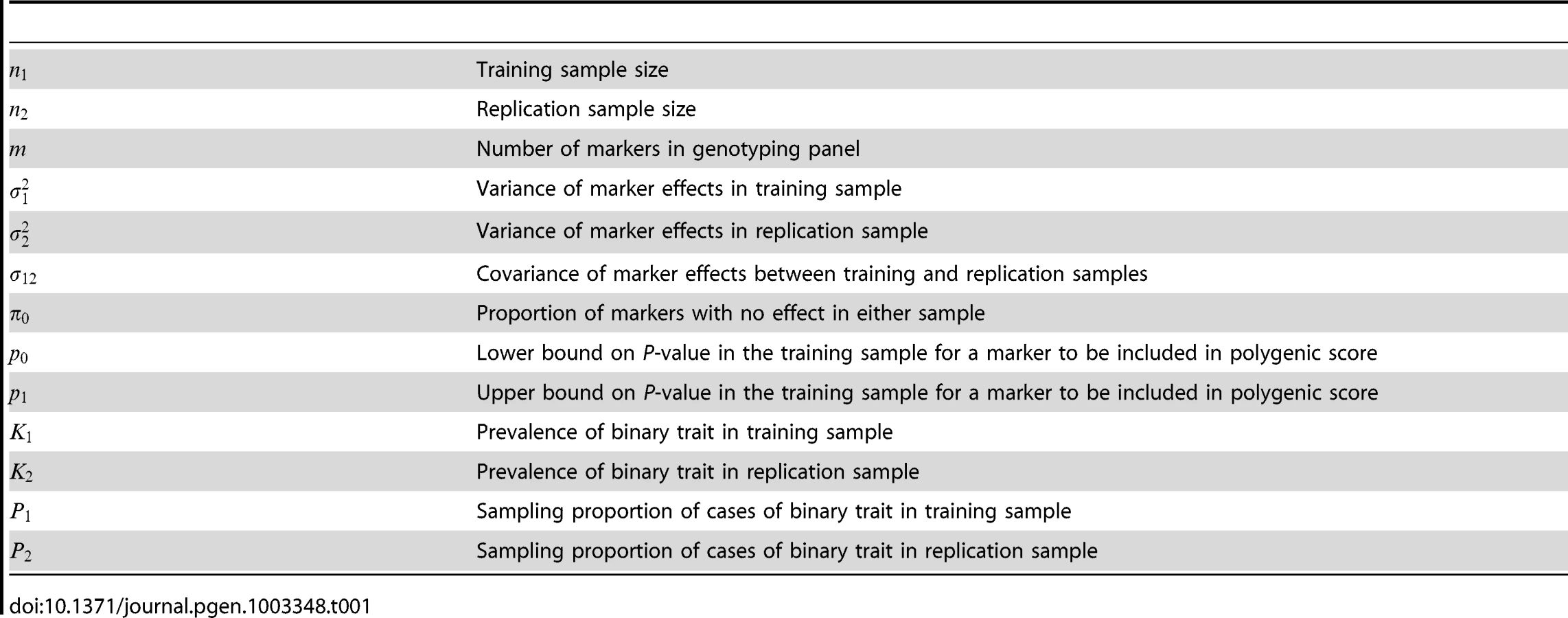
Equation 4 suggests an estimating equation for any parameter of the quantitative model, given the association test between and . Write explicitly as a function of some parameter in Table 1, treating all other parameters as fixed and known. For example, might be the variance of marker effects in the training sample , from which is the explained genetic variance of the marker panel. Alternatively might be the covariance between marker effects in the two samples , assuming fixed values for the explained variances, and so on. Equation 4 is the squared coefficient of the linear regression of on , scaled by its sampling variance. The sampling distribution of that coefficient is normal, with mean the square root of equation 4. Therefore applying normal theory an estimator is the solution to the equation


Published data: Association testing
The ISC was the first to demonstrate the utility of testing polygenic scores [3]. In their main result, odds ratios for 74062 nearly independent SNPs were estimated in 3322 cases and 3587 controls and used to construct a polygenic score that was tested in 2687 cases and 2656 controls of the Molecular Genetics of Schizophrenia study [26]. The score was more strongly associated as higher P-value thresholds were used for including SNPs, with the most significant reported association having with an inclusion threshold of .
Assuming a prevalence of 1%, equation 5 gives a power of 80% at nominal significance if the explained genetic variance in liability is 7.2%, rising to 99% if the explained genetic variance is 11.7%. Assuming a heritability of 80% [3] this shows that the test was well powered if the marker panel explains about 10% of the heritability, which seems reasonable. The observed result of can be used in equation 6 to give an estimated explained genetic variance of 28.7% (95% CI: 23.6%–33.7%), which is 36% of the heritability, assuming that all SNPs have effects that are identical in the two samples. The estimate reduces only to 26.9% if 99% of the SNPs are assumed null. These results are similar to a recent estimate using mixed modelling of the same data [27].
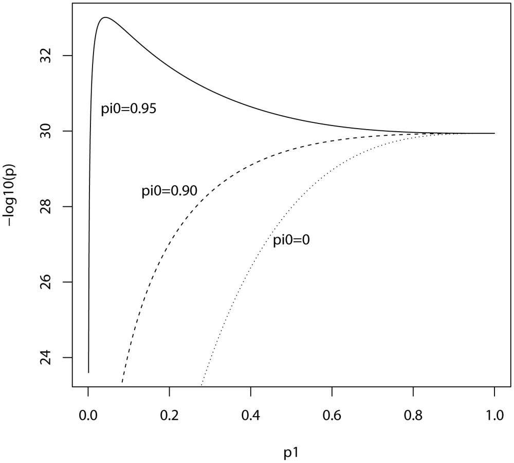
In the ISC report, the P-value of the polygenic score decreases as the SNP inclusion threshold increases. This seems to suggest that a large number of associated markers lie within the mass of individually non-significant SNPs. In Figure 1 and Figure 2, the expected P-value of the polygenic score is shown as a function of the inclusion threshold, with the explained genetic variance set to its estimated value of 28.7% and other parameters as stated above. The figures show that this trend could be observed when as many as 90% of SNPs have no effects, and for the linear regression estimator the significance of the score continues to improve until the whole marker panel is included. Only for a very high proportion of null SNPs is there an optimal inclusion threshold less than 1. The allele count estimator has an optimum threshold less than 1 for all scenarios, but it is consistently less significant. Thus, in this dataset with high power, decreasing P-values are consistent with a range of polygenic models including those with a high proportion of null markers.

In this analysis the replication sample was smaller than the training sample, and we may ask what balance of sample sizes is optimal. Given the total sample size of 3322+2687 = 6009 cases and 3587+2656 = 6243 controls, the non-centrality parameter can be numerically maximised over the proportion of subjects allocated to the training sample. It is found that the optimal split is close to one-half regardless of the proportion of null SNPs or the P-value threshold, and the non-centrality parameter is roughly symmetrical around one-half. This suggests that given two samples of different size, it matters little which is chosen for training and which for testing. Furthermore, given an initial sample to be split into training and replication subsets, an obvious rule of thumb is to make an even split. Similar properties are seen under different genetic models (results not shown). Note that these results apply to association testing and not to individual prediction, which is discussed in the next subsection. For association testing there is a balance to be made between the precision of estimating the score in the training subset, and the power of testing the score in the replication subset. For prediction, however, the size of the replication subset does not affect the accuracy, only how precisely it is estimated; thus a larger training subset is more desirable in the prediction context.
The ISC further tested the schizophrenia-derived score against bipolar disorder, to test for a common genetic basis to those conditions. Their strongest result was with the Wellcome Trust Case-Control Consortium (WTCCC) sample of 1829 cases and 2935 controls, obtaining with an inclusion threshold of . Assume similar heritability for bipolar disorder as for schizophrenia [28] and the same genetic variance explained by the markers, estimated above to be 28.7%. Then using equation 5, the study had 80% power at nominal significance if the correlation is 28% between genetic effects on schizophrenia and bipolar disorder. Using equation 6, the estimated correlation given the observed association statistic is 70.6% (95%CI: 51.3%–89.7%) assuming that all SNPs have effects with explained variance 28.7% in both samples. If 99% of SNPs are assumed null, the estimated correlation reduces to 66.2% (95%CI: 48.1%–84.1%).
The International Multiple Sclerosis Consortium performed a similar exercise using a training sample of 931 cases and 2431 controls, a replication sample of 876 cases and 2077 controls, and a marker panel of 59470 nearly independent SNPs [6]. They also observed decreasing P-values for association as more SNPs were included in the score, obtaining when all SNPs were included. Assuming prevalence of 0.1% this analysis has 80% power at nominal significance for explained genetic variance of 9.4%, and the observed result yields an estimate of 31.5% (95%CI: 24.9%–37.9%) assuming all SNPs have effects.
In applying these ideas to breast and prostate cancers, Machiela et al did not find significant associations of polygenic scores [14]. While this could be explained by the genetic architecture of the diseases, a possible explanation (noted by the authors) is the lower sample size together with the low heritability. Their breast cancer study used a total sample of 2287 subjects, approximately half of which were cases and half controls, which was split into training and testing subsets in a 9∶1 ratio for 10-fold cross-validation. The marker panel consisted of 161,702 nearly independent SNPs. Assuming a prevalence of 3.6% and sibling relative risk of 2.5 [29], this design has only 17% power to detect an association of the polygenic score, even if the markers explain the full heritability. If the sample were split in a 1∶1 ratio, the power would increase to 37%.
Their prostate cancer study had a total of 2277 subjects, approximately half of which were cases, again split in a 9∶1 ratio and a marker panel of 165,508 nearly independent SNPs. Assuming a prevalence of 2.4% and sibling relative risk of 2.8 [29], this design has 19% power if the markers explain the full heritability. If the sample were split in a 1∶1 ratio, the power would be 42%. It is clear that even with the optimistic assumption that the markers explain the full heritability, this study was unlikely to detect an association of the polygenic score for either cancer.
What sample size would have sufficient power to detect association of the polygenic score? For breast cancer the heritability of liability is estimated as 44% [21]. If the marker panel explains half of this heritability, roughly as in the ISC study, then two samples each of 1978 cases and 1978 controls would have 80% power at nominal significance. For prostate cancer the heritability of liability is also 44% and 1766 cases and controls would be required in each sample. For the ISC study, assuming explained genetic variance of 28.7%, 735 cases and controls in each sample are sufficient. Thus it appears that association testing is well powered at current sample sizes if two independent studies are used for training and testing, but less well powered if a single sample is split into two subsets.
As a final example of association testing, this time with a quantitative trait, Simonson et al studied the Framingham Risk Score for cardiovascular disease risk [8]. They also used 10-fold cross-validation of a single sample, giving training samples of 1575 subjects and testing samples of 175 subjects. They used a full set of 250,378 SNPs, which is here assumed to be similar to 100,000 independent SNPs. They first selected SNPs with P-values <0.1 into the score, then selected SNPs with 0.1<P<0.2, then 0.2<P<0.3 and so on, giving ten analyses. Even if the trait is fully heritable and explained by these markers, this analysis has 20% power for the SNPs with P<0.1, reducing with each P-value interval. For 0.4<P<0.5, in which the authors found nominal significance of the score, the power is 6.7%. If all SNPs are included in the score, the power would be 38% if the trait is fully explained by the markers, but under a more conservative model in which the explained genetic variance is 30%, the power is just 8% and increases to 13% under an even split of training and testing samples. Again, splitting a single GWAS sample does not admit high power for testing a polygenic score.
Published data: Risk prediction
In their study of breast and prostate cancers Machiela et al also calculated the AUC for prediction of disease from the polygenic score. Here it is more important for the training sample to be large, ensuring accurate estimation of the score, justifying the 10-fold cross-validation design. Their AUC did not exceed 53% for breast cancer and 56.4% for prostate cancer. Under the same assumptions as above, the analytic AUC is 53.6% for breast cancer if the markers explain the full genetic variance, or 51.8% if they explain half. However if the sample were infinitely large, the AUCs would be 89% and 79% respectively. For prostate cancer, the analytic AUCs are 54.1% if the markers explain the full genetic variance, and 52% if they explain half; for a large sample they would be 90% and 80%. Thus, the low AUCs observed by Machiela et al are compatible with their study design, but they could be considerably higher if a larger training sample were available.
Evans et al considered prediction for the seven diseases of the WTCCC [19]. Approximately 2000 cases were available for each disease, with a common set of 1480 controls, and a marker panel of all SNPs on the Affymetrix 500K chip after quality control and exclusion of previously known loci. As this is the same chip used in the ISC study, it is assumed here that the panel is equivalent to 74062 independent SNPs. Logistic regression and allele score estimators were both used to construct scores, and a series of P-value thresholds from 10−5 to 0.8 were considered.
Table 2 compares the results of Evans et al to the analytic AUC for the diseases without strong MHC effects, using P<0.8 to select SNPs into the score, as that threshold generally gave the highest AUC. At that threshold, the choice of has little bearing on the results unless it is very close to 1, so it is set to 0. Also shown is the maximum AUC possible for each disease, obtained by letting the sample size grow to infinity. Bearing in mind that those authors noticed inflation in AUC for null SNPs, it is again clear that their modest results are compatible with the study design, and more encouraging results might be obtained from a larger sample. The calculations also confirm their observation that the allele count estimator is consistently less accurate than logistic regression; however while the two estimators give similar results at this sample size, more considerable differences emerge in the limit of large samples.
![AUC calculated by Evans et al <em class="ref">[19]</em> compared to analytic values when () marker panel explains half the heritability, or () marker panel explains the full heritability.](https://pl-master.mdcdn.cz/media/cache/media_object_image_large/media/image/2248da41fec36c4cc075a67fdde05c2e.png)
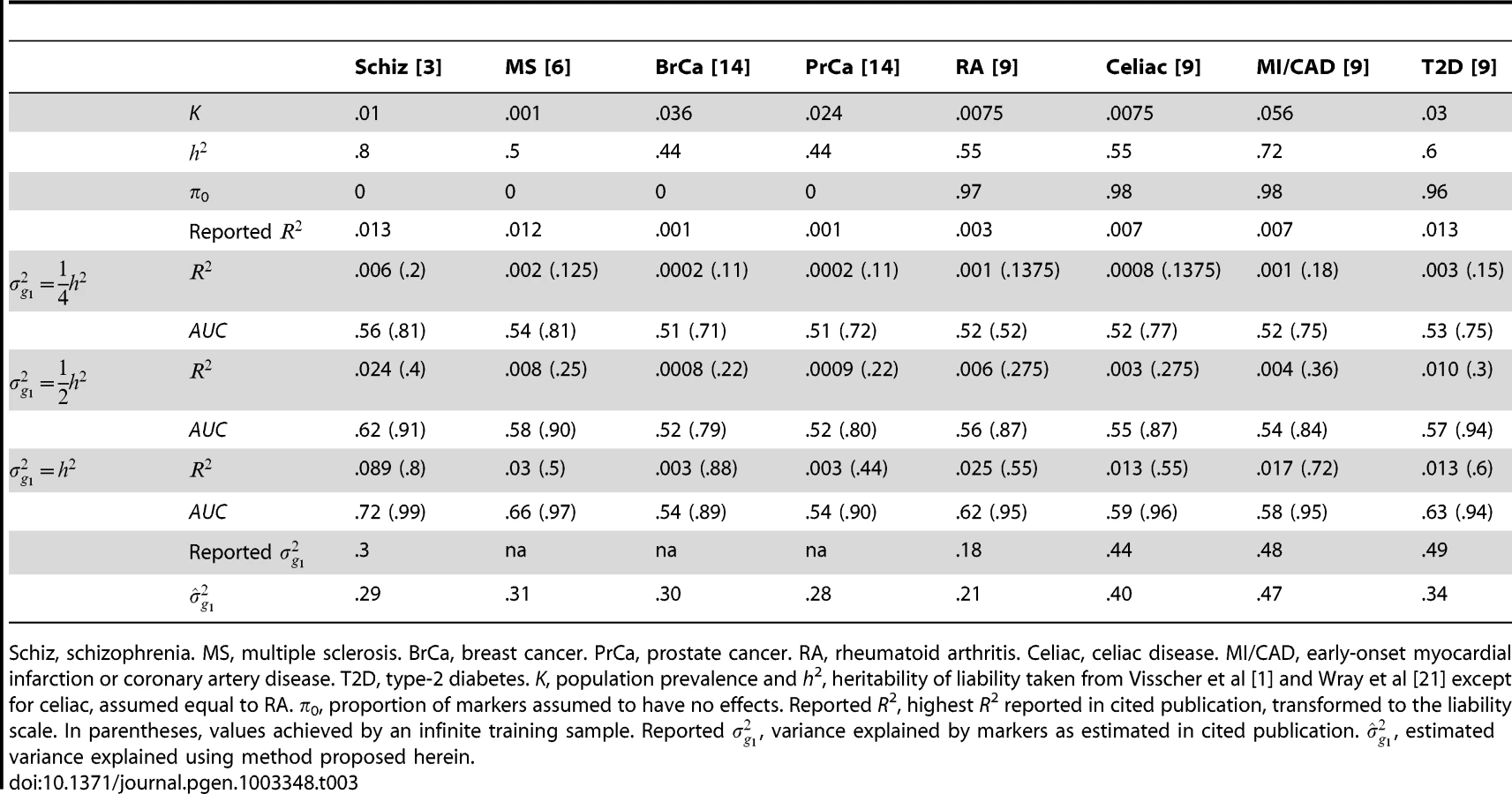
Several other studies have reported pseudo-R2 from the regression of disease on the polygenic score [3], [6], [9]. Although prediction was not emphasised by those studies, they may still be evaluated for that purpose. Recently, Lee et al have argued that, for genetic predictors, R2 on the liability scale is a more interpretable measure of accuracy for binary traits [25]. In Table 3, liability R2 derived from those reports are compared to analytic values assuming different levels of heritability explained by the markers. The choice of has little bearing on these results so it is set to 0 throughout. The reported values are consistent with the markers explaining around half the heritability, with variation above and below. This is in line with the estimates of explained variance that were reported by those studies, and those estimates also agree well with those obtained using the method proposed here (equation 6). The low reported values of R2 do not directly reflect the degree of missing heritability; rather they reflect the effect of sampling variation on the variance explained by an estimated score. Corresponding AUC values are also shown, and it is again clear that the currently modest utility of polygenic scores for discrimination is explained by limited training sample sizes, and much better results are possible through larger samples.
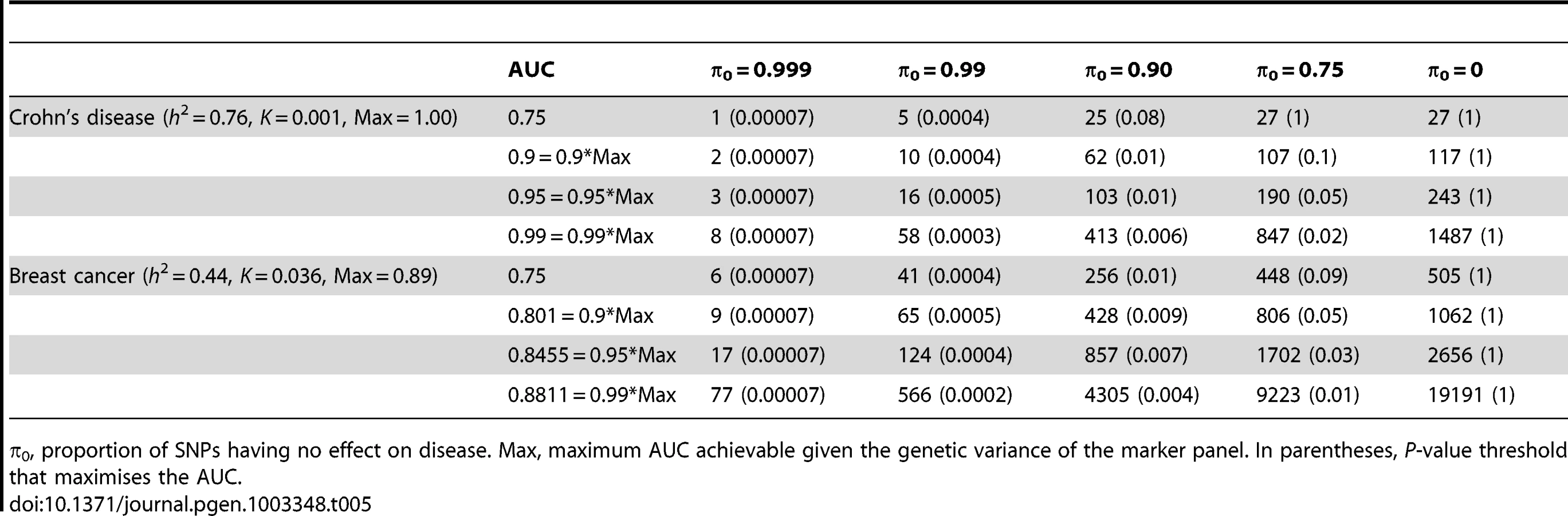
What sample size would permit estimation of a score with AUC at a clinical useful level, or otherwise close to its maximum value? The answer depends on , the proportion of null markers in the panel, because if this is high then the individual marker effects will also be high and a low P-value threshold will eliminate much sampling error from the estimated score. Figure 3 shows AUC as a function of sample size for Crohn's disease, which has a high heritability of 76%, and breast cancer, which has low heritability of 44% [21], based on a panel of 100,000 independent markers. This is a similar number to current genotyping products, and results are given under a scenario in which the panel explains half the heritability [30]. For each sample size and , the P-value threshold is applied that leads to the highest AUC. An AUC of 0.75 is generally regarded as the minimum useful level for screening subjects already considered at risk, whereas AUC of 0.99 is sufficient for screening the population at large [31]. For these two diseases the latter cannot be achieved from genetic data alone, so Table 4 gives minimum sample sizes for AUC of 0.75 and for 90%, 95% and 99% of the maximum possible AUC given the heritability.


The most favourable condition shown is , that is there are 1000 markers with effects on disease. Figure 3 and Table 4 show that a few thousand cases and controls could yield a clinically useful AUC, but under most conditions several tens of thousands are needed. Under less favourable conditions – low heritability, low proportion of null markers – several hundred thousand cases and controls are needed to obtain an AUC within 10% of the achievable level, and even an AUC of 0.75 requires some tens of thousands of subjects. In the worst case the order of magnitude is of the millions.
Whole genome genotyping is now becoming feasible, under which the entire narrow-sense heritability would be represented. Assuming this is equivalent to about one million independent common SNPs [32], the required sample sizes are shown in Figure 4 and Table 5. Again, unless the heritability is explained by about 1000 markers, several tens to hundreds of thousands of subjects are needed to obtain a clinically useful AUC; for the genetic predictor to approach its potential, the order of magnitude is of the millions. The sample sizes to achieve AUC of 0.75 are larger than for 100,000 SNPs explaining half the heritability, but the latter scenario cannot achieve AUC of 0.99, so the clinical context can influence the choice of marker panel used to derive the predictor. It is clear that at current sample sizes, polygenic scores are only going to approach useful levels of discrimination if the marker panels include a high proportion of associated loci and the number of such loci is relatively small. Furthermore, for highly polygenic conditions the sample sizes needed to approach this potential are an order of magnitude higher than are currently available.

Finally, Table 6 gives similar calculations for the correlation between predicted and observed quantitative traits with high (h2 = 0.8) and moderate (h2 = 0.4) heritability. The prospects here appear more challenging in terms of the sample sizes needed to approach the achievable correlation. For example, height has heritability of about 0.8, and the number of associated variants is known to be at least in the hundreds [7]. In the most optimistic scenario shown, 31,000 subjects would be required to derive a predictor with correlation 0.8 with the true height. In fact these sample sizes are now being approached by collaborative studies, and this result confirms that this is necessary for accurate prediction of quantitative traits in addition to the primary goal of identifying individually associated markers.

Discussion
To date polygenic score analyses have been performed opportunistically. The results provided here allow a more informed appraisal of these analyses, characterisation of the statistical properties of the methods, and insights into the future prospects of polygenic modelling. R code to compute the formulae in this paper is available from the author (sites.google.com/site/fdudbridge/software/).
Current sample sizes are clearly adequate for testing association of a polygenic score in a replication sample, as long as full size samples are used for both training and testing. This is already apparent from the extraordinary significance levels reported in the seminal studies [3], [6], but here it is shown that those results are compatible with realistic genetic models and are not necessarily explained by analytic biases that accumulate across SNPs. This had been previously shown by the ISC study, which simulated plausible genetic models and showed that they led to similar results to those observed in the data [3]; here, the result is shown directly for the common quantitative model, without recourse to simulations. Studies that split a single sample into cross-validation subsets have been less successful [8], [14], but here it is shown that this could be explained by their limited sample sizes, and more encouraging results for the same traits could be obtained with modestly increased samples.
When a sample is to be split into two subsets, a roughly even split yields the greatest power for testing association of the score. However, for predicting individual trait values it is more important for the training set to be large, and standard procedures such as 10-fold cross-validation remain preferable. If both testing and prediction are intended from a single sample, a pragmatic approach is to ensure adequate power by allocating about 2000 cases and 2000 controls to the replication sample, providing this is less than half the total, and then to ensure high predictive accuracy by allocating the remainder to the training sample.
The outlook for disease and trait prediction is more challenging. To date the severe shortfall in the accuracy of genetic predictors has generally been ascribed to incomplete coverage of marker panels or failure to identify sufficiently many associated markers. Here, however, no criteria for declaring individual significance are imposed, but neither does the calculation force the predictor to include markers that contribute no information. Under this pragmatic approach it results that tens of thousands of subjects, at least, are needed to derive predictors that are clinically useful. Furthermore, previous results on the potential accuracy of genetic prediction [17], [20]–[22] only become relevant at very large sample sizes. Such numbers are now coming within reach of national biobank projects and international consortia, so the emergence of useful genetic predictors may not be too far off, although such large samples create issues of effect heterogeneity that are not addressed here. Recent estimates of the proportion of markers having effects also suggest that the more optimistic scenarios shown in Table 4, Table 5, Table 6 may apply [9], [33]. Although the focus here is on AUC, various other measures of predictive accuracy are possible and can be computed within the same framework [24], [25]. The expressions given here could be adapted to other measures without much difficulty.
For some diseases, fairly high AUC has already been observed [17], [19]. This does not conflict with the present work but reflects the presence of major gene effects, usually in the MHC, which depart from the quantitative model treated here. Similarly, some diseases have non-genetic risk factors that already admit clinically useful predictors. There the more relevant issue is the extent to which genetics improves established models [34]. Again the focus has tended to lie on identifying specific markers to improve prediction, rather than the sample size needed to accurately estimate their combined effects. The approach taken here could easily be extended to accommodate additional fixed effects.
A fairly general construction of the polygenic score has been described, including weighted and unweighted methods from single marker analysis, and shrinkage methods used in multivariate analysis. There is little to choose between these estimators in terms of power, correlation or AUC, but the unweighted estimator will perform relatively worse as sample size increases since its sampling error does not reduce to zero. Shrinkage estimation leads to reduced mean square error for prediction and has some other advantages [35], [36], but in the main applications for polygenic scores to date, namely association testing and AUC, it does not improve over the linear regression estimate.
However, some ideal conditions have been assumed including independence of markers and of study subjects. In reality markers will be in linkage disequilibrium and the approximation by an effective number of independent tests is heuristic. Similarly, subjects will be related, if distantly. Results from real data may depart from those presented here if proper account is taken of relationships between subjects. In particular, shrinkage estimation is likely to improve power and correlation, as well as mean square error, by analysing all markers simultaneously rather than each one marginally [37].
The assumption that effects are normally distributed is necessary when markers are selected by their P-values but not otherwise. Similarly, allowing a proportion of markers to have no effect only makes a difference when selecting markers by P-values. Thus the present results are relevant even if one does not entirely accept the polygenic model proposed. The normal distribution simplifies some calculations, but various heavy-tailed distributions have also been proposed for GWAS data [38], [39] and would lead to improved prediction if such models held in truth. Furthermore the assumption of normality applies to effects on the standardised genotype scale, but there are plausible models for effect sizes as a function of allele frequency, leading to non-normal effects on the standardised scale. This may particularly affect the results for shrinkage estimation when the degree of shrinkage varies for markers with different allele frequencies. The numerical results presented are therefore not definitive but should be taken a guide to the likely magnitude of results in specific applications.
A novel approach to estimating parameters of the polygenic model has been proposed, showing promise for inferring the explained genetic variance and/or proportion of null markers. The method yields estimates that are similar to those obtained by existing approaches [1], [37]. A similar approach to estimation has been developed by Stahl et al [9], based on simulating GWAS data from proposed models, and using rejection sampling to construct posterior distributions of their parameters. Apart from the accommodation of prior distributions (which were uninformative), this is essentially the same approach as used here except that whole genome simulation is used to obtain a sampling distribution. The analytic results provided here should allow this approach to be implemented more efficiently, and this will be attempted in future work.
The P-value thresholds that maximise the power and AUC are more permissive than the usual thresholds for individual markers. This means that polygenic analyses can be powerful while still including many non-significant markers, so they will continue to be useful as long as individually associated markers remain to be discovered. Although larger samples are needed for useful risk prediction, polygenic scores have an ongoing current role in assessing the variance explained by marker panels and the genetic correlation between related traits and populations.
Methods
Quantitative model
Recall equation 1 in which a pair of traits is expressed as a linear combination of genetic effects and an error term that includes environmental and unmodelled genetic effects:


The genetic effects on are estimated from a sample of size and used to construct a polygenic score to be tested for association to in an independent sample of size . Define the polygenic score to be


Equations 2–6 in Results follow immediately, in which the key quantities are and . They in turn depend upon the form of the estimator , for which three alternatives are now discussed.
Linear regression
A natural estimate of is the least squares estimate from the univariate linear regression of on . Then is asymptotically normally distributed with sampling mean and variance since is standardised by definition. Assuming that genetic effects are small, it is henceforth conservatively taken that as previously suggested by Daetwyler et al [23]. The total variance of this estimator over markers and samples is , and its correlation with the effects on is


Now suppose markers are only selected into the polygenic score if they have two-tailed P-values between thresholds where . Asymptotically the equivalent constraint for is obtained from the Wald statistic as

Suppose further that a proportion of the markers have no effect on (ie. ), and the remaining markers have effects drawn from . Then among the null markers the variance of , conditional on selection into the polygenic score, is obtained from properties of the truncated normal distribution as [40]


To obtain allowing for selection of markers, note that the regression of on has the same coefficient regardless of selection on . For non-null markers this coefficient is


Shrinkage estimation
It is well known that estimation and prediction for multivariate models can be improved, in terms of mean squared error, by assuming that their effects come from a common underlying distribution. A common approach in quantitative genetics is to fit a mixed model in which genetic markers have random effects for which best linear unbiased predictors (BLUPs) are obtained [35]. This is one of several closely related formulations of multilevel models [36]. As these approaches tend to give similar results when the number of markers is large, a basic Bayesian estimation scheme is outlined here and will be assumed to give typical results for a shrinkage estimator.
Suppose has the prior distribution , and let the “data” consist of the univariate linear regression estimates, . Then the posterior for given is also normal, where [41]. A natural estimator for is therefore the posterior mean for which and . Since all effects are shrunk by the same factor it follows that this approach leads to the same power and correlation as the linear regression estimator , but the mean square error is reduced to .
Allele count
A currently common approach is to construct the polygenic score by summing the number of trait-increasing alleles across selected markers, without considering their effect sizes other than to identify the direction of association at each marker. This may be called an unweighted score, in contrast to the above approaches that estimate weights for each marker. The unweighted score may be more robust against errors in estimating the effect sizes arising from limited sample size, population heterogeneity, “winner's curse” bias, and confounding by population structure. Here a related approach is considered in which all markers are given the same absolute effect size on the standardised genotype scale. This is equivalent to the allele counting approach when all markers have the same allele frequency. When allele frequencies are heterogeneous, allele counting assumes that all markers have the same effect on the trait, whereas the present approach assumes that all markers contribute the same proportion of variance to the trait. Both models can be criticised but the present approach will allow the comparison of weighted to unweighted scores without considering the distribution of allele frequencies or their relation to the effect sizes.
The polygenic score is now calculated as


Binary traits
The forgoing is based on linear regression, which is the usual approach for quantitative traits. For binary traits the standard analysis is logistic regression, used both for estimating the coefficients in the polygenic score and for testing the association of the score in a replication sample. For small effects the log-odds are approximately linear in the predictors, so we may continue to work in a linear regression framework for estimating power and accuracy. That is, the binary trait is coded as 0/1 and treated as the response in ordinary linear regression. The variance of in equation 2 is now the binomial variance where is the proportion of study subjects with . In a prospective sample, is the population proportion of the trait, whereas in a case/control sample (to be discussed further below), it is the sampling proportion of cases.
The binary traits are now assumed to arise from a liability threshold model, under which all individuals have an underlying normally distributed trait, called the liability, and all those whose liability exceeds a fixed threshold will exhibit the trait. Although the liability is not directly observed, this model has several advantages for modelling polygenic effects, including independence of the genetic effects from the trait prevalence, and an elegant linear transformation between effects on liability to corresponding effects on the observed (0/1) trait. This model has recently been elucidated by several authors for studying the quantitative genetics of binary traits in humans, and the reader is referred to their papers for more detailed discussion [21], [24], [30].
Assuming the marginal liabilities are distributed as a standard normal, the threshold for exhibiting trait is where is the population prevalence. The genetic effects are now taken to act on liability, and for small effects a linear transformation to the corresponding effect on the observed trait may be obtained as [30]

Sensitivity and specificity are often of interest in the prediction of binary traits. In particular, the accuracy of a predictor can be assessed by the AUC constructed as follows. Subjects are classified such that those with a polygenic score above a fixed threshold are predicted to have the trait, those below the threshold to not have it. Sensitivity is the proportion of subjects with the trait who are correctly predicted as such, and specificity the proportion of subjects without the trait correctly predicted as such. Each possible threshold leads to a value of sensitivity and specificity, defining the receiver operator characteristic curve by plotting sensitivity against 1-specificity. The AUC can be defined as the probability that a pair of subjects, one with the trait and one without, is correctly classified by the predictor. Because the central limit theorem implies that the polygenic score is normally distributed, the expected AUC can be calculated as [21]


Case/control studies
In case/control studies the increased ascertainment of cases leads to departure from the normal distribution of liability assumed in the previous subsection. To overcome this problem, it is again assumed that there is a linear transformation from an effect on liability to one on the observed trait in which the 0/1 response denotes ascertained case status.
When there is no selection on or the regression of on has coefficient from equation 11. The converse regression of on has coefficient . The latter will also apply when there is ascertainment on , but the regression of on ascertained can also be written as , where denotes ascertainment, so that


To obtain the AUC, the same approach as before is used, but now using


Liability R2
The derived expressions involve which is the coefficient of determination on the observed scale. Lee et al have argued that, for a genetic predictor, R2 on the liability scale is more interpretable for binary traits as it is invariant to the population prevalence and sampling ratio [25]. An approximate transformation to the liability scale is obtained by transforming the genetic effects using equation 13 and rescaling the trait variance from the binomial variance on the observed scale to the unit variance on the liability scale. Therefore,

Log-risk model
An alternative to the liability threshold model is the log-risk model for binary traits, which is equivalent to the logistic model in the limit of low prevalence. Here the polygenic score estimates the log risk of disease, which is assumed to be normally distributed in the population with mean and variance , where is the sibling relative recurrence risk [17], [20]. Under this model the log risk has the same variance in cases and controls, but the mean log risk among cases is increased by that same variance, becoming . This model allows a simpler calculation of AUC for rare disease, which is given here but not pursued further.
Given and and denoting log-risk of trait by , the transformation from log-risk to observed scales is


Simulations
The derived expressions were compared to simulations in which the major assumptions were examined under realistic scenarios. These assumptions include a large number of markers with effects, for equality in equation 7, and small genetic effects, so that effects on the liability scale are approximately linear. In case/control designs the disease prevalence is assumed to be not too small, so that the variance of the ascertained genotypes remains near 1 as assumed in equation 13 and Text S1. Effects are assumed to be normally distributed on the standardised genotype scale. Sample sizes are assumed large so that estimates of genetic effects are normally distributed.
A baseline scenario was defined to reflect that seen in recent studies, as follows. Two normally distributed traits were simulated with explained genetic variances 0.4 and 0.3 and correlation of genetic effects of 0.65. Genotypes from 100,000 independent SNPs were simulated, with minor allele frequencies uniformly distributed on (0.01, 0.5). This reflects current marker panels that directly explain about half the heritability [1]. The proportion of null SNPs was 0.95 or 0.99 [9], with the same SNPs having effects for both traits. Their effect sizes were drawn from the bivariate normal distribution such that the desired variances and covariance were attained. The traits were then generated from the quantitative model in equation 1.
The polygenic score was estimated using the first trait in a sample of 4000 unrelated subjects. The score was constructed using P-value thresholds of 0.1 and 0.001 for π0 = 0.95 and 0.99 respectively; these thresholds yielded the highest R2 and AUC values. The score was then tested for association with the second trait in an independent sample of 4000 subjects. The correlation and mean square error between the score and the second trait were also estimated in the second sample. The association tests were used in equation 6 to estimate the explained genetic variances in the first and second samples in turn, and then the covariance between effects in the two samples, each time keeping other parameters fixed to their simulation values.
Table S1 shows estimates from 1000 simulations compared to the analytic values, for the three estimators discussed. Mean square error for the allele count estimator is not meaningful without further scaling of the polygenic score, which is a further problem not of present interest. All simulations agree well with the analytic results. Because the variances and covariance are bounded in (0,1), their median estimates are shown with the coverage, rather than their means. The proposed estimating equations are seen to be accurate, but the confidence intervals are anti-conservative when the number of markers with effects is low, here 1000. This is because the realised variance and covariance in equation 7 depart from their large m expectation, with resulting over-dispersion in the estimating equation (left hand side of equation 6). However when the number of markers with effects is 5000, the correct coverage is attained.
The traits were then treated as liabilities for binary diseases with prevalence 0.2. Disease status was simulated prospectively, as in a cohort study. The polygenic score was estimated and tested using both linear and logistic regression. Table S2 shows estimates of power and AUC compared to the analytic values. Results for the shrinkage estimator are identical to the regression estimator and are not shown. All simulations agree well with the analytic results, and the proposed estimating equations are accurate. The results for logistic regression agree well with those for linear regression, justifying the use of the latter to derive the analytic results.
Then, a case/control design was simulated in which the disease prevalence was now 0.001. The same total sample sizes were used but included equal numbers of cases and controls. A computationally efficient approach to this simulation is described in Text S2. The results are given in Table S3. Again all simulations are seen to agree with the analytic values, but when the number of markers with effects is low, there is a downward bias in the parameter estimates and the confidence intervals of the parameter estimates are anti-conservative. Again the logistic regression results agree well with those for linear regression. Taking Tables S1, S2, S3 together, the analytic methods are accurate for the strongest effects likely to be seen in current studies, but when the number of SNPs with effects is about 1000, there is downward bias in the effect estimates and under-coverage of the confidence intervals, the degree of which appears to vary with the strength of the association.
To assess robustness to normality of the marker effects, the simulations were repeated with the effects drawn from Laplace distributions and then rescaled to give the same explained variance and correlation as before. Instead of π0 = 0.95 and P<0.1, simulations with π0 = 0 and P<1 were performed to verify that this situation does not assume normality. The results in Table S4, Table S5 and Table S6 confirm this to be the case, whereas when π0 = 0.99 and P<0.001 the analytic expressions tend to underestimate the power and accuracy. This is due to the heavier tails of the Laplace distribution compared to the normal, and quantitatively different results would be seen for different generating models. Again, bias and under-coverage is seen when there are 1000 markers with effects.
Supporting Information
Zdroje
1. VisscherPM, BrownMA, McCarthyMI, YangJ (2012) Five years of GWAS discovery. Am J Hum Genet 90 : 7–24.
2. WrayNR, GoddardME, VisscherPM (2007) Prediction of individual genetic risk to disease from genome-wide association studies. Genome Res 17 : 1520–1528.
3. PurcellSM, WrayNR, StoneJL, VisscherPM, O'DonovanMC, et al. (2009) Common polygenic variation contributes to risk of schizophrenia and bipolar disorder. Nature 460 : 748–752.
4. RipkeS, SandersAR, KendlerKS, LevinsonDF, SklarP, et al. (2011) Genome-wide association study identifies five new schizophrenia loci. Nat Genet 43 : 969–976.
5. HamshereML, O'DonovanMC, JonesIR, JonesL, KirovG, et al. (2011) Polygenic dissection of the bipolar phenotype. Br J Psychiatry 198 : 284–288.
6. BushWS, SawcerSJ, de JagerPL, OksenbergJR, McCauleyJL, et al. (2010) Evidence for polygenic susceptibility to multiple sclerosis–the shape of things to come. Am J Hum Genet 86 : 621–625.
7. Lango AllenH, EstradaK, LettreG, BerndtSI, WeedonMN, et al. (2010) Hundreds of variants clustered in genomic loci and biological pathways affect human height. Nature 467 : 832–838.
8. SimonsonMA, WillsAG, KellerMC, McQueenMB (2011) Recent methods for polygenic analysis of genome-wide data implicate an important effect of common variants on cardiovascular disease risk. BMC Med Genet 12 : 146.
9. StahlEA, WegmannD, TrynkaG, Gutierrez-AchuryJ, DoR, et al. (2012) Bayesian inference analyses of the polygenic architecture of rheumatoid arthritis. Nat Genet 44 : 483–489.
10. SpeliotesEK, WillerCJ, BerndtSI, MondaKL, ThorleifssonG, et al. (2010) Association analyses of 249,796 individuals reveal 18 new loci associated with body mass index. Nat Genet 42 : 937–948.
11. PetersonRE, MaesHH, HolmansP, SandersAR, LevinsonDF, et al. (2011) Genetic risk sum score comprised of common polygenic variation is associated with body mass index. Hum Genet 129 : 221–230.
12. CarayolJ, SchellenbergGD, ToresF, HagerJ, ZieglerA, et al. (2010) Assessing the impact of a combined analysis of four common low-risk genetic variants on autism risk. Mol Autism 1 : 4.
13. KangJ, KugathasanS, GeorgesM, ZhaoH, ChoJH (2011) Improved risk prediction for Crohn's disease with a multi-locus approach. Hum Mol Genet 20 : 2435–2442.
14. MachielaMJ, ChenCY, ChenC, ChanockSJ, HunterDJ, et al. (2011) Evaluation of polygenic risk scores for predicting breast and prostate cancer risk. Genet Epidemiol 35 : 506–514.
15. WitteJS, HoffmannTJ (2011) Polygenic modeling of genome-wide association studies: an application to prostate and breast cancer. OMICS 15 : 393–398.
16. PharoahPD, AntoniouAC, EastonDF, PonderBA (2008) Polygenes, risk prediction, and targeted prevention of breast cancer. N Engl J Med 358 : 2796–2803.
17. ClaytonDG (2009) Prediction and interaction in complex disease genetics: experience in type 1 diabetes. PLoS Genet 5: e1000540 doi:10.1371/journal.pgen.1000540
18. SawcerS, BanM, WasonJ, DudbridgeF (2010) What role for genetics in the prediction of multiple sclerosis? Ann Neurol 67 : 3–10.
19. EvansDM, VisscherPM, WrayNR (2009) Harnessing the information contained within genome-wide association studies to improve individual prediction of complex disease risk. Hum Mol Genet 18 : 3525–3531.
20. PharoahPD, AntoniouA, BobrowM, ZimmernRL, EastonDF, et al. (2002) Polygenic susceptibility to breast cancer and implications for prevention. Nat Genet 31 : 33–36.
21. WrayNR, YangJ, GoddardME, VisscherPM (2010) The genetic interpretation of area under the ROC curve in genomic profiling. PLoS Genet 6: e1000864 doi:10.1371/journal.pgen.1000864
22. JanssensAC, AulchenkoYS, ElefanteS, BorsboomGJ, SteyerbergEW, et al. (2006) Predictive testing for complex diseases using multiple genes: fact or fiction? Genet Med 8 : 395–400.
23. DaetwylerHD, VillanuevaB, WoolliamsJA (2008) Accuracy of predicting the genetic risk of disease using a genome-wide approach. PLoS ONE 3: e3395 doi:10.1371/journal.pone.0003395
24. SoHC, ShamPC (2010) A unifying framework for evaluating the predictive power of genetic variants based on the level of heritability explained. PLoS Genet 6: e1001230 doi:10.1371/journal.pgen.1001230
25. LeeSH, GoddardME, WrayNR, VisscherPM (2012) A better coefficient of determination for genetic profile analysis. Genet Epidemiol 36 : 214–224.
26. ShiJ, LevinsonDF, DuanJ, SandersAR, ZhengY, et al. (2009) Common variants on chromosome 6p22.1 are associated with schizophrenia. Nature 460 : 753–757.
27. LeeSH, DeCandiaTR, RipkeS, YangJ, SullivanPF, et al. (2012) Estimating the proportion of variation in susceptibility to schizophrenia captured by common SNPs. Nat Genet 44 : 247–250.
28. SklarP, RipkeS, ScottLJ, AndreassenOA, CichonS, et al. (2011) Large-scale genome-wide association analysis of bipolar disorder identifies a new susceptibility locus near ODZ4. Nat Genet 43 : 977–983.
29. RischN (2001) The genetic epidemiology of cancer: interpreting family and twin studies and their implications for molecular genetic approaches. Cancer Epidemiol Biomarkers Prev 10 : 733–741.
30. LeeSH, WrayNR, GoddardME, VisscherPM (2011) Estimating missing heritability for disease from genome-wide association studies. Am J Hum Genet 88 : 294–305.
31. JanssensAC, MoonesingheR, YangQ, SteyerbergEW, van DuijnCM, et al. (2007) The impact of genotype frequencies on the clinical validity of genomic profiling for predicting common chronic diseases. Genet Med 9 : 528–535.
32. DudbridgeF, GusnantoA (2008) Estimation of significance thresholds for genomewide association scans. Genet Epidemiol 32 : 227–234.
33. YangJ, WeedonMN, PurcellS, LettreG, EstradaK, et al. (2011) Genomic inflation factors under polygenic inheritance. Eur J Hum Genet 19 : 807–812.
34. WacholderS, HartgeP, PrenticeR, Garcia-ClosasM, FeigelsonHS, et al. (2010) Performance of common genetic variants in breast-cancer risk models. N Engl J Med 362 : 986–993.
35. GoddardME, WrayNR, VerbylaK, VisscherPM (2009) Estimating Effects and Making Predictions from Genome-Wide Marker Data. Statistical Science 24 : 517–529.
36. GreenlandS (2000) Principles of multilevel modelling. Int J Epidemiol 29 : 158–167.
37. YangJ, BenyaminB, McEvoyBP, GordonS, HendersAK, et al. (2010) Common SNPs explain a large proportion of the heritability for human height. Nat Genet 42 : 565–569.
38. WuTT, ChenYF, HastieT, SobelE, LangeK (2009) Genome-wide association analysis by lasso penalized logistic regression. Bioinformatics 25 : 714–721.
39. HoggartCJ, WhittakerJC, De IorioM, BaldingDJ (2008) Simultaneous analysis of all SNPs in genome-wide and re-sequencing association studies. PLoS Genet 4: e1000130 doi:10.1371/journal.pgen.1000130
40. Falconer DS, Mackay TFC (1996) Introduction to Quantitative Genetics: Longman.
41. Ruppert D, Wand MP, Carroll RJ (2003) Semiparametric regression: Cambridge University Press.
Štítky
Genetika Reprodukční medicínaČlánek vyšel v časopise
PLOS Genetics
2013 Číslo 3
- Kazuistika – Perspektivy využití precizované medicíny v rámci personalizované specifické terapie onkologických pacientů
- Nobelova cena za chemii pro genetické nůžky: Objev, který změní naši budoucnost?
- Technologie na bázi RNA v klinické praxi: od přebarvených petúnií k terapii vzácných a dosud jen obtížně léčitelných chorob u lidí
- „Nepředstavovali jsme si, že náš výzkum povede přímo ke vzniku nových léků, dokonce ještě za našeho života“
- Bezplatné služby pro diagnostiku ATTRv amyloidózy pro kardiology
Nejčtenější v tomto čísle
- Fine Characterisation of a Recombination Hotspot at the Locus and Resolution of the Paradoxical Excess of Duplications over Deletions in the General Population
- Molecular Networks of Human Muscle Adaptation to Exercise and Age
- Recurrent Rearrangement during Adaptive Evolution in an Interspecific Yeast Hybrid Suggests a Model for Rapid Introgression
- Genome-Wide Association Study and Gene Expression Analysis Identifies as a Predictor of Response to Etanercept Therapy in Rheumatoid Arthritis
Zvyšte si kvalifikaci online z pohodlí domova
Mazová zátka a její řešení
nový kurzVšechny kurzy